James E. Pustejovsky – Investigating selective reporting in meta-analyses of dependent effect sizes

Collaborators from the American Institutes for Research

Martyna Citkowicz

Megha Joshi

Ryan Williams

Joshua Polanin

Melissa Rodgers

David Miller

Acknowledgement

The research reported here was supported, in whole or in part, by the Institute of Education Sciences, U.S. Department of Education, through grant R305D220026 to the American Institutes for Research. The opinions expressed are those of the authors and do not represent the views of the Institute or the U.S. Department of Education.

Selective reporting of primary study results

Selective reporting occurs if affirmative findings are more likely to be reported and available for inclusion in meta-analysis
Selective reporting can distort the evidence base available for systematic review/meta-analysis
- Inflate average effect size estimates from meta-analysis
- Bias estimates of heterogeneity (Augusteijn, van Aert, and van Assen 2019)
Strong concerns about selective reporting across social, behavioral, and health sciences.

Many available tools for investigating selective reporting

Graphical diagnostics
- Funnel plots
- Contour-enhanced funnel plots
- Power-enhanced funnel plots (sunset plots)

Tests/adjustments for funnel plot asymmetry
- Trim-and-fill
- Egger’s regression
- PET/PEESE
- Kinked meta-regression
Selection models
- Weight-function models
- Copas models
- Sensitivity analysis
p-value diagnostics
- Test of Excess Significance
- $p$ -curve / $p$ -uniform / $p {-uniform}^{*}$

But few that accommodate dependent effect sizes

Dependent effect sizes are ubiquitous in education and social science meta-analyses.
We have well-developed methods for modeling dependent effect sizes assuming no selection.
But only very recent developments for investigating selective reporting in databases with dependent effect sizes (Chen and Pustejovsky 2024).

Extending step-function selection models

Location-scale-selection regressions
Alternative estimation methods
Handling dependence
Simulation findings

Step-function selection models

The data for $j = 1, . . ., J$ studies with $i = 1, . . ., k_{j}$ effect size estimates
- $T_{i j}, σ_{i j}$ estimate and standard error for effect size $i$ from study $j$
- $p_{i j} = Φ^{- 1} (- T_{i j} / σ_{i j})$ one-sided $p$ -value of estimate $i$ from study $j$ .

Random effects model for the evidence-generating process (before selective reporting): $T_{i j} \sim N (μ, τ^{2} + σ_{i j}^{2})$

Vevea and Hedges (1995) $H$ -step model for the selection process with steps $α_{1}, . . ., α_{H}$ (taking $λ_{0} = 1, α_{0} = 0, α_{H + 1} = 1$ ): $Pr (T_{i j} is observed) \propto \sum_{h = 0}^{H} λ_{h} \times I (α_{h} \leq p_{i j} < α_{H + 1})$

A piece-wise normal distribution

The step-function model implies that the distribution of observed effect size estimates is piece-wise normal.

math = require("mathjs")
norm = import('https://unpkg.com/norm-dist@3.1.0/index.js?module')

eta = math.sqrt(tau**2 + sigma**2)
H = 2
alpha = [alpha1, alpha2]
lambda = [1, lambda1, lambda2_ratio * lambda1]
lambda_max = math.max(lambda)

function findlambda(p, alp, lam) {
  var m = 0;
  while (p >= alp[m]) {
    m += 1;
  }
  return lam[m];
}

function findMoments(mu, tau, sigma, alp, lam) {
  let H = alp.length;
  let eta = math.sqrt(tau**2 + sigma**2);
  
  let gamma_h = Array(H+2).fill(null).map((x,i) => {
    if (i==0) {
      return Infinity;
    } else if (i==H+1) {
      return -Infinity;
    } else {
      return sigma * norm.icdf(1 - alp[i-1]);
    }
  });
  
  let c_h = Array(H+2).fill(null).map((x,i) => {
    return (gamma_h[i] - mu) / eta;
  });

  let B_h = Array(H+1).fill(null).map((x,i) => {
    return norm.cdf(c_h[i]) - norm.cdf(c_h[i+1])
  });

  let Ai = 0;
  for (let i = 0; i <= H; i++) {
    Ai += lam[i] * B_h[i];
  }
  
  let psi_h = Array(H+1).fill(null).map((x,i) => {
    return (norm.pdf(c_h[i+1]) - norm.pdf(c_h[i])) / B_h[i]
  }); 

  let psi_top = 0;
  for (let i = 0; i <= H; i++) {
    psi_top += lam[i] * B_h[i] * psi_h[i];
  }
  
  let psi_bar = psi_top / Ai;

  let ET = mu + eta * psi_bar;

  let dc_h = c_h.map((c_val) => {
    if (math.abs(c_val) == Infinity) {
      return 0;
    } else {
      return c_val * norm.pdf(c_val);
    }
  });

  let kappa_h = Array(H+1).fill(null).map((x,i) => {
    return (dc_h[i] - dc_h[i+1]) / B_h[i];
  });

  let kappa_top = 0;
  for (let i = 0; i <= H; i++) {
    kappa_top += lam[i] * B_h[i] * kappa_h[i];
  }
  let kappa_bar = kappa_top / Ai;
  let SDT = eta * math.sqrt(1 - kappa_bar - psi_bar**2);
  
  return ({Ai: Ai, ET: ET, SDT: SDT});
}

moments = findMoments(mu, tau, sigma, alpha, lambda)
Ai_toprint = moments.Ai.toFixed(3)
ET_toprint = moments.ET.toFixed(3)
eta_toprint = eta.toFixed(3)
SDT_toprint = moments.SDT.toFixed(3)

math = Object {isNumber: ƒ(e), isComplex: ƒ(e), isBigNumber: ƒ(e), isBigInt: ƒ(e), isFraction: ƒ(e), isUnit: ƒ(e), isString: ƒ(e), isArray: ƒ(), isMatrix: ƒ(e), isCollection: ƒ(e), isDenseMatrix: ƒ(e), isSparseMatrix: ƒ(e), isRange: ƒ(e), isIndex: ƒ(e), isBoolean: ƒ(e), isResultSet: ƒ(e), isHelp: ƒ(e), isFunction: ƒ(e), isDate: ƒ(e), isRegExp: ƒ(e), …}

norm = Module {Z: ƒ(…), cdf: ƒ(z), icdf: ƒ(…), intE: ƒ(a, b), pdf: ƒ(z), Symbol(Symbol.toStringTag): "Module"}

eta = 0.291547594742265

H = 2

alpha = Array(2) [0.025, 0.5]

lambda = Array(3) [1, 1, 1]

lambda_max = 1

findlambda = ƒ(p, alp, lam)

findMoments = ƒ(mu, tau, sigma, alp, lam)

moments = Object {Ai: 1, ET: 0.1, SDT: 0.291547594742265}

Ai_toprint = "1.000"

ET_toprint = "0.100"

eta_toprint = "0.292"

SDT_toprint = "0.292"

pts = 201

density_dat = Array(pts).fill().map((element, index) => {
  let t = mu - 3 * eta + index * eta * 6 / (pts - 1);
  let p = 1 - norm.cdf(t / sigma);
  let dt = norm.pdf((t - mu) / eta) / eta;
  let lambda_val = findlambda(p, alpha, lambda);
  return ({
    t: t,
    d_unselected: dt,
    d_selected: lambda_val * dt / lambda_max
  })
})

pts = 201

density_dat = Array(201) [Object, Object, Object, Object, Object, Object, Object, Object, Object, Object, Object, Object, Object, Object, Object, Object, Object, Object, Object, Object, …]

viewof mu = Inputs.range(
  [-2, 2], 
  {value: 0.1, step: 0.01, label: tex`\mu`}
)

viewof tau = Inputs.range(
  [0, 2], 
  {value: 0.15, step: 0.01, label: tex`\tau`}
)

viewof sigma = Inputs.range(
  [0, 1], 
  {value: 0.25, step: 0.01, label: tex`\sigma_i`}
)

viewof alpha1 = Inputs.range(
  [0, 1],
  {value: 0.025, step: 0.005, label: tex`\alpha_1`}
)

viewof alpha2 = Inputs.range(
  [0, 1],
  {value: 0.50, step: 0.005, label: tex`\alpha_2`}
)

viewof lambda1 = Inputs.range(
  [0, 2],
  {value: 1, step: 0.01, label: tex`\lambda_1`}
)

viewof lambda2_ratio = Inputs.range(
  [0, 2],
  {value: 1, step: 0.01, label: tex`\lambda_2 / \lambda_1`}
)

mu = 0.1

tau = 0.15

sigma = 0.25

alpha1 = 0.025

alpha2 = 0.5

lambda1 = 1

lambda2_ratio = 1

Plot.plot({
  height: 500,
  width: 1000,
  y: {
    grid: false,
    label: "Density"
  },
  x: {
    label: "Effect size estimate (Ti)"
  },   
  marks: [
    Plot.ruleY([0]),
    Plot.ruleX([0]),
    Plot.areaY(density_dat, {x: "t", y: "d_unselected", fillOpacity: 0.3}),
    Plot.areaY(density_dat, {x: "t", y: "d_selected", fill: "blue", fillOpacity: 0.5}),
    Plot.lineY(density_dat, {x: "t", y: "d_selected", stroke: "blue"})
  ]
})

tex`
\begin{aligned}
\mu &= ${mu} & \qquad \sqrt{\tau^2 + \sigma_{ij}} &= ${eta_toprint} \\
\mathbb{E}\left(T_{ij}\right) &= ${ET_toprint}
& \qquad \sqrt{\mathbb{V}\left(T_{ij}\right)} &= ${SDT_toprint} \\ 
\Pr(T_{ij} \text{ is observed}) &= ${Ai_toprint}
\end{aligned}
`

\begin{aligned} \mu &= 0.1 & \qquad \sqrt{\tau^2 + \sigma_{ij}} &= 0.292 \\ \mathbb{E}\left(T_{ij}\right) &= 0.100 & \qquad \sqrt{\mathbb{V}\left(T_{ij}\right)} &= 0.292 \\ \Pr(T_{ij} \text{ is observed}) &= 1.000 \end{aligned}

Location-scale-selection meta-regressions

Viechtbauer and López‐López (2022) proposed location-scale meta-regression: $\begin{aligned} T_{i j} & \sim N (μ_{i j}, τ_{i j}^{2} + σ_{i j}^{2}) \\ μ_{i j} & = x_{i j} β \\ \log (τ_{i j}^{2}) & = u_{i j} γ \end{aligned}$

We use the location-scale model as the evidence-generating process.

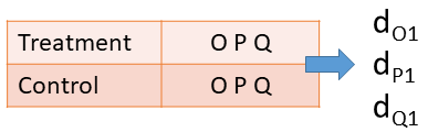
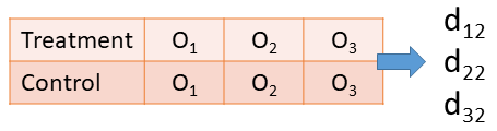
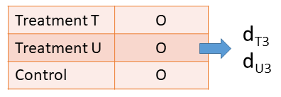
We allow selection parameters to vary according to predictors: $\begin{aligned} Pr (T_{i j} is observed) & \propto \sum_{h = 0}^{H} λ_{h i j} \times I (α_{h} \leq p_{i j} < α_{H + 1}) \\ \log (λ_{h i j}) & = z_{i j}^{(h)} ζ_{h} \end{aligned}$

Why allow varying selection parameters?

Coburn and Vevea (2015) investigated variation in strength of selection as a function of study characteristics.
- Meta-scientific questions about how selective reporting changes over time, as a result of intervention, or by outcome type.
- Change in selection process could act as a confounder of real secular changes.

Account for studies that follow reporting practices that are not susceptible to selective reporting (Van Aert 2025).
- Pre-registered reports are assumed to be fully reported.
- A selection regression with no intercept:
$\log (λ_{h i j}) = 0 + ζ_{h} \times I (Not Pre-Reg.)_{i j}$

Color priming

Lehmann, Elliot, and Calin-Jageman (2018) reported a systematic review of studies on color-priming, examining whether exposure to the color red influenced attractiveness judgements.

Many published studies where selective reporting was suspected.
Review included 11 pre-registered studies.

	Mean ES		Heterogeneity Variance
Coef.	Est.	SE	Est.	SE
(A) Summary meta-analysis
Overall	0.2073	0.0571	0.1032	0.0251
(B) Moderation by study type
Pre-Registered	-0.0456	0.0407	0.0959	0.024
Not Pre-Registered	0.2504	0.0633	0.0959	0.024

	Mean ES		Heterogeneity Variance
Coef.	Est.	SE	Est.	SE
(A) Summary meta-analysis
Overall	0.2073	0.0571	0.1032	0.0251
(B) Moderation by study type
Pre-Registered	-0.0456	0.0407	0.0959	0.024
Not Pre-Registered	0.2504	0.0633	0.0959	0.024

Color-priming selection models

	Mean ES		Heterogeneity Variance		Selection Parameter
Coef.	Est.	SE	Est.	SE	Est.	SE
(A) Summary selection model
Overall	0.1328	0.1373	0.0811	0.0845	0.548	0.616
(B) Mean moderation by study type
Pre-Registered	-0.0854	0.0587	0.0738	0.0776	0.547	0.606
Not Pre-Registered	0.2591	0.1173	0.0738	0.0776	0.547	0.606
(C) Selective Reporting of Non-Pre-Registered Studies
Pre-Registered	0.1031	0.0966	0.0723	0.0756	1	-
Not Pre-Registered	0.1031	0.0966	0.0723	0.0756	0.366	0.369

	Mean ES		Heterogeneity Variance		Selection Parameter
Coef.	Est.	SE	Est.	SE	Est.	SE
(A) Summary selection model
Overall	0.1328	0.1373	0.0811	0.0845	0.548	0.616
(B) Mean moderation by study type
Pre-Registered	-0.0854	0.0587	0.0738	0.0776	0.547	0.606
Not Pre-Registered	0.2591	0.1173	0.0738	0.0776	0.547	0.606
(C) Selective Reporting of Non-Pre-Registered Studies
Pre-Registered	0.1031	0.0966	0.0723	0.0756	1	-
Not Pre-Registered	0.1031	0.0966	0.0723	0.0756	0.366	0.369

	Mean ES		Heterogeneity Variance		Selection Parameter
Coef.	Est.	SE	Est.	SE	Est.	SE
(A) Summary selection model
Overall	0.1328	0.1373	0.0811	0.0845	0.548	0.616
(B) Mean moderation by study type
Pre-Registered	-0.0854	0.0587	0.0738	0.0776	0.547	0.606
Not Pre-Registered	0.2591	0.1173	0.0738	0.0776	0.547	0.606
(C) Selective Reporting of Non-Pre-Registered Studies
Pre-Registered	0.1031	0.0966	0.0723	0.0756	1	-
Not Pre-Registered	0.1031	0.0966	0.0723	0.0756	0.366	0.369

Estimation

Model the marginal distribution of observed effects, ignoring the dependence structure

Composite marginal likelihood: $\arg max_{β, γ, ζ} \prod_{j = 1}^{J} \prod_{i = 1}^{k_{j}} L (T_{i j} | x_{i j}, u_{i j}, z_{i j}; β, γ, ζ)$

Augmented, reweighted Gaussian likelihood:

$\arg max_{β, γ} \sum_{j = 1}^{J} \sum_{i = 1}^{k_{j}} \frac{\log N (x_{i j} β, \exp (u_{i j} γ) + σ_{i j}^{2})}{Pr (T_{i j} is observed | β, γ, ζ)}$ such that $\sum_{j = 1}^{J} \sum_{i = 1}^{k_{j}} I (λ_{h} < p_{i j} \leq λ_{h + 1}) = \sum_{j = 1}^{J} \sum_{i = 1}^{k_{j}} Pr (λ_{h} < P_{i j} \leq λ_{h + 1} | β, γ, ζ)$

Two methods of handling dependence

CML and ARGL estimators do not directly account for dependent effect sizes.

Cluster-robust variance estimation (sandwich estimators)

Clustered bootstrap re-sampling
- percentile, studentized, or BCa confidence intervals

Simulation Study

Data-generating process

Simulated summary statistics for two-group comparison designs with multiple, correlated continuous outcomes. Correlated-and-hierarchical effects generating process:

$\begin{aligned} δ_{i j} & = μ + u_{i} + v_{i j}, u_{i} \sim N (0, τ^{2}), v_{i j} \sim N (0, ω^{2}) \\ T_{j} & \sim N (δ_{j}, \frac{4}{N_{j}} ((1 - ρ) I_{j} + ρ J_{j})) \end{aligned}$
Varying primary study sample sizes $N_{j}$ and varying numbers of outcomes $k_{j}$ , based on large database of impact evaluation studies in education research.
Censored one-sided $p$ -values > .025 with probability of selection $0 < λ_{1} \leq 1$

Comparison estimators
- Correlated-and-hierarchical effects (CHE) model
- PET-PEESE regression adjustment with cluster-robust SEs

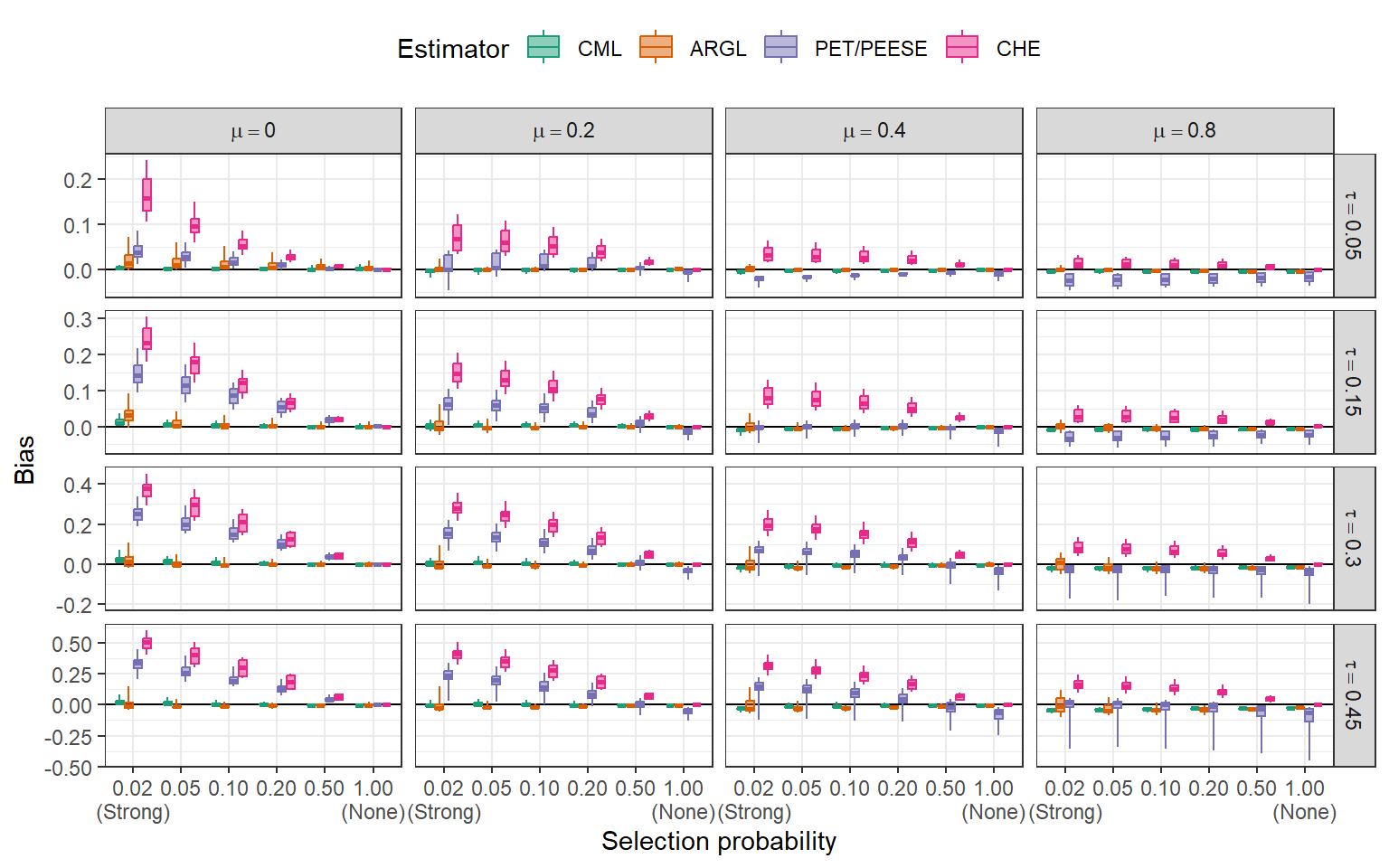
Bias for mean effect size $(μ)$

viewof mu_bias = Inputs.input(0.0)
viewof tau_bias = Inputs.input(0.15)

bias_dat = transpose(dat).filter(function(el) {
  return el.mean_smd == mu_bias && el.tau == tau_bias;
})

viewof mu_bias = EventTarget {value: 0}

mu_bias = 0

viewof tau_bias = EventTarget {value: 0.15}

tau_bias = 0.15

bias_dat = Array(960) [Object, Object, Object, Object, Object, Object, Object, Object, Object, Object, Object, Object, Object, Object, Object, Object, Object, Object, Object, Object, …]

Inputs.bind(
  Inputs.select(
    [0.0,0.2,0.4,0.8], 
    {
      value: 0.0, 
      label: tex`\mu`,
      width: "100px"
    }
  ),
  viewof mu_bias
)

Inputs.bind(
  Inputs.select(
    [0.05,0.15,0.30,0.45], 
    {
      value: 0.15, 
      label: tex`\tau`,
      width: "100px"
    }
  ),
  viewof tau_bias
)

Plot.plot({
  x: {
    domain: ["CML","ARGL","PET/PEESE","CHE"],
    label: null,
    axis: null
  },
  fill: {
    domain: ["CML","ARGL","PET/PEESE","CHE"],
  },
  y: {
    grid: true,
    domain: [-0.1,0.4]
  },
  fx: {
    padding: 0.10,
    label: "Selection probability",
    labelAnchor: "center"
  },
  width: 800,
  height: 500,
  color: {
    domain: ["CML","ARGL","PET/PEESE","CHE"],
    legend: true
  },
  marks: [
    Plot.ruleY([0.0], {stroke: "black"}),
    Plot.boxY(bias_dat, {fx: "weights", x: "estimator", y: "bias", stroke: "estimator", fill: "estimator"})
  ]
})

CMLARGLPET/PEESECHE

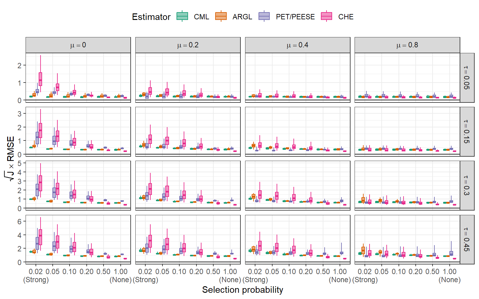
Accuracy for mean effect size $(μ)$

Inputs.bind(
  Inputs.select(
    [0.0,0.2,0.4,0.8], 
    {
      value: 0.0, 
      label: tex`\mu`,
      width: "100px"
    }
  ),
  viewof mu_bias
)

Inputs.bind(
  Inputs.select(
    [0.05,0.15,0.30,0.45], 
    {
      value: 0.15, 
      label: tex`\tau`,
      width: "100px"
    }
  ),
  viewof tau_bias
)

Plot.plot({
  x: {
    domain: ["CML","ARGL","PET/PEESE","CHE"],
    label: null,
    axis: null
  },
  fill: {
    domain: ["CML","ARGL","PET/PEESE","CHE"],
  },
  y: {
    grid: true,
  },
  fx: {
    padding: 0.10,
    label: "Selection probability",
    labelAnchor: "center"
  },
  width: 800,
  height: 500,
  color: {
    domain: ["CML","ARGL","PET/PEESE","CHE"],
    legend: true
  },
  marks: [
    Plot.ruleY([0.0], {stroke: "black"}),
    Plot.boxY(bias_dat, {fx: "weights", x: "estimator", y: "scrmse", stroke: "estimator", fill: "estimator"})
  ]
})

CMLARGLPET/PEESECHE

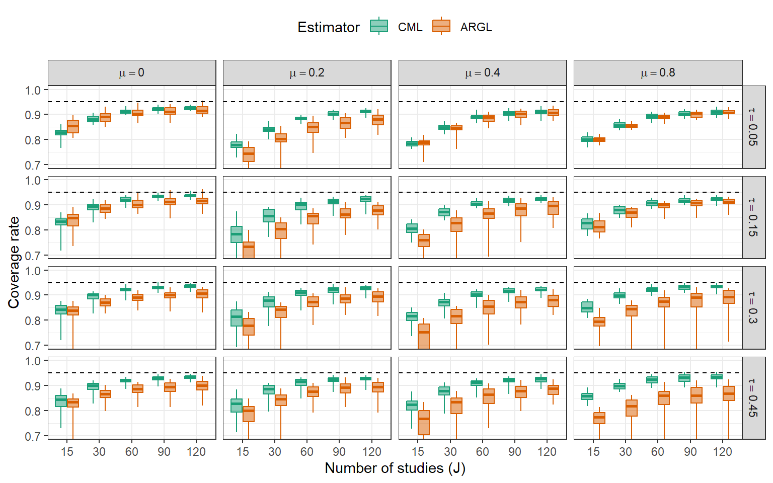
Coverage rates of 95% CIs for $μ$

coverage_dat = transpose(CI_dat).filter(function(el) {
  return el.mean_smd == mu_CI && el.tau == tau_CI && estimator.includes(el.estimator);
})

coverage_dat = Array(108) [Object, Object, Object, Object, Object, Object, Object, Object, Object, Object, Object, Object, Object, Object, Object, Object, Object, Object, Object, Object, …]

viewof mu_CI = Inputs.select(
    [0.0,0.4,0.8], 
    {
      value: 0.0, 
      label: tex`\mu`,
      width: "100px"
    }
  )

viewof tau_CI = Inputs.select(
    [0.05,0.15,0.30,0.45], 
    {
      value: 0.05, 
      label: tex`\tau`,
      width: "100px"
    }
  )

viewof estimator = Inputs.select(
    ["CML","ARGL"], 
    {
      value: "CML", 
      label: "estimator",
      width: "100px"
    }
  )

mu_CI = 0

tau_CI = 0.05

estimator = "CML"

Plot.plot({
  x: {
    axis: null
  },
  y: {
    grid: true,
    domain: [0.70,1.00]
  },
  fx: {
    padding: 0.10,
    label: "Number of studies (J)",
    labelAnchor: "center"
  },
  color: {
    legend: true
  },
  width: 800,
  height: 500,
  marks: [
    Plot.ruleY([0.95], {stroke: "black", strokeDasharray: "5,3"}),
    Plot.boxY(coverage_dat, {fx: "J", x: "CI_boot_method", y: "coverage", stroke: "CI_boot_method", fill: "CI_boot_method"})
  ]
})

cluster-robustpercentile (multinomial)

Discussion

Marginal step-function selection models are worth adding to the toolbox.
- Low bias compared to other selective reporting adjustments (including PET-PEESE)
- Bias-variance trade-off relative to regular meta-analytic models
- Clustered bootstrap percentile confidence intervals work tolerably well

Marginal modeling costs precision
- Further development should consider estimators that handle dependence (pairwise composite likelihood?)

Selective reporting of each outcome
- Our data-generating process involved conditional independence of $Pr (T_{i j} is observed | p_{i j})$
- Need further models (and diagnostics) for multivariate selection processes

R package `metaselection`

Currently available on Github at https://github.com/jepusto/metaselection
Install using

remotes::install_github("jepusto/metaselection", build_vignettes = TRUE)
Under active development, suggestions welcome!

References

Augusteijn, Hilde E. M., Robbie C. M. van Aert, and Marcel A. L. M. van Assen. 2019. “The Effect of Publication Bias on the Q Test and Assessment of Heterogeneity.” Psychological Methods 24 (1): 116–34. https://doi.org/10.1037/met0000197.

Chen, Man, and James E. Pustejovsky. 2024. “Adapting Methods for Correcting Selective Reporting Bias in Meta-Analysis of Dependent Effect Sizes.” https://doi.org/10.31222/osf.io/jq52s.

Coburn, Kathleen M, and Jack L Vevea. 2015. “Publication bias as a function of study characteristics.” Psychological Methods 20 (3): 310–30. https://doi.org/10.1037/met0000046.

Lehmann, Gabrielle K, Andrew J Elliot, and Robert J Calin-Jageman. 2018. “Meta-Analysis of the Effect of Red on Perceived Attractiveness.” Evolutionary Psychology 16 (4): 1474704918802412.

Van Aert, Robbie C. M. 2025. “Meta-Analyzing Nonpreregistered and Preregistered Studies.” Psychological Methods, February. https://doi.org/10.1037/met0000719.

Vevea, Jack L, and Larry V Hedges. 1995. “A General Linear Model for Estimating Effect Size in the Presence of Publication Bias.” Psychometrika 60 (3): 419–35. https://doi.org/10.1007/BF02294384.

Viechtbauer, Wolfgang, and José Antonio López‐López. 2022. “Location‐scale Models for Meta‐analysis.” Research Synthesis Methods, April, jrsm.1562. https://doi.org/10.1002/jrsm.1562.

Supplementary Material

Simulation Design

Parameter	Full Simulation	Bootstrap Simulation
Overall average effect	0.0, 0.2, 0.4, 0.8	0.0, 0.2, 0.4, 0.8
Between-study heterogeneity	0.05, 0.15, 0.30, 0.45	0.05, 0.45
Within-study heterogeneity ratio	0.0, 0.5	0.0, 0.5
Correlation between outcomes	0.4, 0.8	0.8
Selection probability	0.02, 0.05, 0.10, 0.20, 0.50, 1.00	0.05, 0.20, 1.00
Number of primary studies	15, 30, 60, 90, 120	15, 30, 60
Primary study sample sizes	Typical, Small	Typical, Small

2000 replications per condition
399 bootstraps per replication