---
title: Meta-Analysis of Variance for Monte Carlo Simulations
date: '2026-07-31'
categories:
- distribution theory
- experimental design
- simulation
code-fold: true
code-tools: true
toc: true
bibliography: "../simulation.bib"
csl: "../apa.csl"
link-citations: true
---
Monte Carlo simulation studies are a workhorse of quantitative methodology.
Whether you are developing new methods, trying to understand existing ones, or figuring out how to do a nuanced analysis of some empirical data, simulations are useful and widely used in practice.
One reason that simulations are so useful for investigating methodological questions is that they provide a practical complement to theoretical analysis. Theory is, for one, hard and, for another, often limited to broad, approximate results (as $N \to \infty$) or special cases (...assume all schools have the same number of students...).
In contrast, simulations are relatively easy to conduct (even if your math is rusty) and informative about _particular_ and _specific_ circumstances.
Simulations are such a central, everyday part of my work that [Megha Joshi](/people/Megha-Joshi/) and I [developed an R package](/software/simhelpers/) to support coding them up, and [Luke Miratrix](https://cares.gse.harvard.edu/about-luke-miratrix) are writing [a textbook](https://jepusto.github.io/Designing-Simulations-in-R/) about how to do them.
Considering just how important and routine simulations are for our work, statisticians and methodologists are often surprisingly casual about analyzing the results.
Often, results are reported in giant, gnarly tables that make it difficult to identify any broader patterns.[^Gelman]
In my own work and in collaborative work with students or colleagues, I typically present results using graphical visualizations---often, _many_ of them---that make heavy use of small multiples (i.e., `facet_grid()` in `ggplot2`) to represent different dimensions of the simulation.[^interactive]
But these presentations are still fairly informal, putting much of the onus on the reader / viewer to interpret the patterns.
Shouldn't there be more _statistical_ ways of analyzing simulations? Shouldn't we methodologists be walking the walk, practicing what we preach, and eating our own dogfood, so to speak?
[^Gelman]: Many years ago, @Gelman2002lets called out several articles in the Journal of the American Statistical Association for presenting results in poorly constructed tables, arguing that graphical presentations are nearly always superior.
[^interactive]: Recently, I've been playing with interactive figures, as in [this example](/posts/Displaying-simulation-results/).
Simulations are designed experiments, often following a full factorial design.
Thus, one would think that classical analysis of variance (ANOVA) would be an obvious tool for analysis of simulation experiments.[^Harwell]
My students and I have used this approach in some simulation studies [e.g., @lee2024comparing] and found it to be quite useful.
In our work, we use ANOVA as a first-pass analysis, to get an initial sense of which factors in our design are driving variation in the performance of a method.
This is quite useful for figuring out where to dig in further and how to construct figures to represent the results clearly.
But our interpretation of ANOVAs has relied more strongly than I would like on borrowed conventions (like partial $\eta^2$ effect sizes) and informal judgments.
It would be great to bring a little bit more rigor to how we use ANOVA in the context of simulations.
[^Harwell]: In a survey of simulations published in statistics and biostatistics journals, @Harwell2018survey found that this is very uncommon, with less than 1% of articles reporting ANOVA of simulation reports.
I'm not going to do that in one blog post, of course.
In this post, I want to tackle one specific aspect of how to do ANOVA on simulation results: how to handle Monte Carlo error.
For a given performance measure, ANOVA tables involve sums-of-squares of the variation in performance attributable to different factors and combinations of factors.
Because we're dealing with simulation results, the performance measures have Monte Carlo error in them, and so sums-of-squares will be due in part to actual variation and in part just to the Monte Carlo error.
It would be nice to pull those two sources apart.
## An example
Here's an example to illustrate the problem. As I mentioned, @lee2024comparing used ANOVA to get oriented to the factors influencing the performance of a set of methods.
For context, the paper is about how to analyze cross-classified random effects models and what happens when some assumptions of those models are violated.
The simulation was a five-factor experiment in a fully crossed design, involving manipulation of:
1. Assumption violations (4 levels, labelled $a$)
2. Magnitude of a focal regression coefficient (3 levels, labelled $b$),
3. Number of higher-level units in each dimension of the cross-classification (3 levels, labelled $H$),
4. Number of lower-level units per higher-level unit (2 levels, labelled $J$), and
5. Degree of intra-class correlation in each dimension (3 levels, labelled).
Under each of the 216 conditions, we estimated a cross-classified random effects model (CCREM), a simpler ordinary least squares regression that ignores the random effects structure, and a two-way fixed effects regression. For simplicity, I will focus on the performance of the CCREM estimator of the sole lower-level predictor in the model.
```{r setup}
#| echo: false
library(tinytable)
```
```{r}
#| output: false
library(tidyverse)
load(here::here("data","Lee-Pustejovsky-2023-simulation-results.Rdata"))

CCREM_res <-
  results %>%
  filter(method == "CCREM", cov == "X") %>%
  mutate(
    a = as.factor(assumption),
    b = as.factor(gamma100),
    H = as.factor(H),
    J = as.factor(J),
    ICC = as.factor(ICC_h),
    rmse = 100 * rmse,
    rmse_mcse = 100 * rmse_mcse
  )

aov_fit <- aov(rmse ~ a * b * H * J * ICC, data = CCREM_res)
summary(aov_fit)
```
```{r}
#| echo: false
#| label: tbl-Lee-ANOVA
#| tbl-cap: Analysis of Variance Table for Root Mean Squared Error of the CCREM estimator
aov_table <-
summary(aov_fit)[[1]] %>%
as_tibble(rownames = "term")
aov_table %>%
tt() %>%
format_tt(digits = 2, num_fmt = "decimal") %>%
style_tt(j = 2:4, align = "r") %>%
theme_striped()
```
@tbl-Lee-ANOVA displays a full factorial ANOVA for the root mean squared error (RMSE) of the CCREM estimator, summarizing the extent to which each of these factors and their interactions explains variation in RMSE across the conditions.
It's clear just from looking at the table that $a$ and $H$ are the only factors that explain much variation in RMSE.
But what about the variation attributed to the remaining components?
How much of it is just Monte Carlo error?
To answer this question, let me formalize the problem.
## Meta-ANOVA
Suppose we have a performance measure $\Upsilon$ (bias, RMSE, confidence interval coverage, etc.) evaluated under each condition in a full factorial design.
I'll assume that there are five factors in all (just as in my example), with $m_A$, $m_B$, $m_C$, $m_D$, and $m_Z$ levels, respectively.
For condition $abcdz$, we use simulation to compute an estimate of $\Upsilon_{abcdz}$, denoted $y_{abcdz}$, with associated Monte Carlo error $\sigma_{abcdz}$.
We can think of this as a simple, fixed effect meta-analysis:
$$
\newcommand{\Prob}{\text{Pr}}
\newcommand{\E}{\mathbb{E}}
\newcommand{\M}{\mathbb{M}}
\newcommand{\Q}{\mathbb{Q}}
\newcommand{\Var}{\mathbb{V}}
\newcommand{\Bias}{\text{Bias}}
\newcommand{\RMSE}{\text{RMSE}}
\newcommand{\Cov}{\text{Cov}}
\newcommand{\cor}{\text{cor}}
\newcommand{\diag}{\text{diag}}
\newcommand{\mat}[1]{\mathbf{#1}}
\newcommand{\bs}{\boldsymbol}
\newcommand{\trace}{\text{tr}}
y_{abcdz} = \Upsilon_{abcdz} + \epsilon_{abcdz}, \qquad \text{where} \qquad \epsilon_{abcdz} \sim N\left(0, \ \sigma_{abcdz}^2\right).
$$
A full factorial ANOVA involves a re-parameterization of this model into a set of components corresponding to main effects and interactions:
$$
\begin{aligned}
y_{abcdz} &= \mu + \alpha_a + \beta_b + \gamma_c + \delta_d + \zeta_z & \text{(intercept and main effects)} \\
& \quad + (\alpha\beta)_{ab} + (\alpha\gamma)_{ac} + \cdots & \text{(2-way interactions)} \\
& \quad \quad + (\alpha\beta\gamma)_{abc} + (\alpha\beta\delta)_{abd} + \cdots & \text{(3-way interactions)} \\
& \quad \quad \quad + (\alpha\beta\gamma\delta)_{abcd} + (\alpha\beta\gamma\zeta)_{abcz} + \cdots & \text{(4-way interactions)}\\
& \quad \quad \quad \quad + (\alpha\beta\gamma\delta\zeta)_{abcdz} + \epsilon_{abcdz}. & \text{(5-way interactions)}
\end{aligned}
$$
The target parameters in an ANOVA are sums of the squared coefficients for a particular component.
For instance, the parameter for the two-way interaction between the first two factors is
$$
\Psi_{\alpha\beta} = \sum_{a=1}^{m_A} \sum_{b = 1}^{m_B} \sum_{c = 1}^{m_C} \sum_{d = 1}^{m_D} \sum_{z = 1}^{m_Z} (\alpha\beta)_{ab}^2 = m_C m_D m_Z \sum_{a=1}^{m_A} \sum_{b = 1}^{m_B} (\alpha\beta)_{ab}^2.
$$
In an ANOVA table like @tbl-Lee-ANOVA, the sums of squares are computed by substituting coefficient estimates in place of the parameters.
In using coefficient estimates to compute sums of squares, part of the variation captured will be due to Monte Carlo error.
My goal here is to figure out how much and to subtract it out, yielding an unbiased estimator of the sum of squares attributable to the component.
## Adjusted sums of squares
For purposes of derivation, it's more useful to write the ANOVA model with a different represent that may be more familiar from regression analysis.
Let $q$ index all of the terms in the ANOVA, from first-order (main effects) through the fifth-order interactions.
With five factors, there are a total of $Q = `{r} sum(choose(5,1:5))`$ terms in all.
(More generally, there are a total of $Q = 2^K - 1$ terms in a $K$-factor design.)
Let $\mat{X}_q$ denote the contrast matrix and $\bs\theta_q$ denote the vector of effects for term $q$, with $\mat{X}_0 = \mat{1}$ and $\theta_0 = \mu$. The full model is then
$$
\mat{Y} = \bs\Upsilon + \bs\epsilon = \sum_{q=0}^Q \mat{X}_q \bs\theta_q + \bs\epsilon,
$$
where $\mat{Y} = \left[y_{abcdz}\right]$, $\bs\Upsilon = \left[\Upsilon_{abcdz}\right]$, and $\bs\epsilon = \left[\epsilon_{abcdz}\right]$ are the vectors of outcomes, expectations, and Monte Carlo errors, respectively.
The error vector is normally distributed with mean zero and variance $\bs\Sigma = \bigoplus \ \sigma_{abcdz}^2$.
In a full factorial design, the contrast matrices are all orthogonal. Consequently, $\mat{X}_q' \mat{X}_r = \mat{0}$ for all pairs of terms where $q \neq r$.
Because of orthogonality, the target parameter for component $q$ is simply
$$
\Psi_q = \bs\theta_q' \mat{X}_q'\mat{X}_q \bs\theta_q.
$$
Also because of orthogonality, the estimated coefficients associated with term $q$ are just
$$
\bs{\hat\theta}_q = \left(\mat{X}_q'\mat{X}_q\right)^{-1} \mat{X}_q' \mat{Y}
$$
and the sum of squares for term $q$ is
$$
SS_{q} = \bs{\hat\theta}_q'\mat{X}_q'\mat{X}_q\bs{\hat\theta}_q = \mat{Y}'\mat{X}_q \left(\mat{X}_q'\mat{X}_q\right)^{-1} \mat{X}_q' \mat{Y}.
$$
For compactness, let me write $\mat{P}_q = \mat{X}_q \left(\mat{X}_q'\mat{X}_q\right)^{-1/2}$, so that $SS_q = \mat{Y}'\mat{P}_q \mat{P}_q' \mat{Y}$. Also let $\bs\Omega_q = \mat{P}_q' \bs\Sigma \mat{P}_q$ and $\bs\beta_q = \mat{P}_q'\bs\Upsilon = \left(\mat{X}_q' \mat{X}_q\right)^{1/2} \bs\theta_q$. From standard properties of quadratic forms,
$$
\begin{aligned}
\E\left(SS_q\right) &= \trace\left(\mat{P}_q \mat{P}_q'\bs\Sigma \right) + \bs\Upsilon'\mat{P}_q \mat{P}_q' \bs\Upsilon \\
&= \trace\left(\mat{P}_q' \bs\Sigma \mat{P}_q\right) + \bs\theta_q' \mat{X}_q'\mat{X}_q \bs\theta_q \\
&= \trace\left(\bs\Omega_q\right) + \Psi_q.
\end{aligned}
$$
An unbiased estimator for $\Psi_q$ (the sum of squared effects attributable to term $q$) is then
$$
SSA_q = SS_q - \trace\left(\bs\Omega_q\right).
$$
Also from standard properties of quadratic forms,
$$
\begin{aligned}
\Var\left(SS_q\right) &= 2\trace\left(\mat{P}_q \mat{P}_q' \bs\Sigma \mat{P}_q \mat{P}_q' \bs\Sigma \right) + 4\bs\Upsilon'\mat{P}_q \mat{P}_q' \bs\Sigma \mat{P}_q \mat{P}_q' \bs\Upsilon \\
&= 2\trace\left(\bs\Omega_q \bs\Omega_q \right) + 4\bs\beta_q' \bs\Omega_q \bs\beta_q.
\end{aligned}
$$
A feasible estimator of $\Var(SS_q)$ can be computed by substituting the estimated effects $\bs{\hat\theta}_q$ in place of the parameter vector $\bs\theta_q$, or equivalently by using $\mat{b}_q = \mat{P}_q' \mat{Y}$ in place of $\bs\beta_q$.
Now, in a classical ANOVA, the sums of squares are all mutually independent because the errors are homoskedastic.
That is not the case here, though, and so it's possible that there is some covariance between different terms.
The covariance is
$$
\begin{aligned}
\Cov\left(SS_q, SS_r\right) &= 2\trace\left(\mat{P}_q \mat{P}_q' \bs\Sigma \mat{P}_r \mat{P}_r' \bs\Sigma \right) +4 \bs\Upsilon'\mat{P}_q\mat{P}_q' \bs\Sigma \mat{P}_r \mat{P}_r' \bs\Upsilon \\
&= 2\trace\left(\bs\Omega_{qr} \bs\Omega_{qr}' \right) + 4 \bs\beta_q' \bs\Omega_{qr} \bs\beta_r,
\end{aligned}
$$
where $\bs\Omega_{qr} = \mat{P}_q' \bs\Sigma \mat{P}_r$.
One thing that you might want to do with these results is to test whether the sum of squares for a particular component is zero (as you do with $F$ tests in classical analysis of variance).
So the null here is that $\bs\theta_q = \mat{0}$ for component $q$. Under this null, $\E\left(SS_q\right) = \trace\left(\bs\Omega_q\right)$ and $\Var\left(SS_q\right) = 2\trace\left(\bs\Omega_q\bs\Omega_q\right)$.
Following a Satterthwaite approximation, let $C_q = SS_q / \trace\left(\bs\Omega_q\right)$ and $\nu_q = \left[\trace\left(\bs\Omega_q\right)\right]^2 / \trace\left(\bs\Omega_q\bs\Omega_q\right)$. Then under the null, an approximate reference distribution for the test statistic is $C_q \stackrel{\cdot}{\sim} \chi^2(\nu_q)$.
If $\bs\Omega_q$ is close to a multiple of an identity matrix, then $\nu_q$ will be close to the degrees of freedom for the component.
## Residual sum of squares
So far, I've been assuming that the ANOVA is fully saturated, meaning that every possible factor and interaction among factors is included.
None of the derivations require this, though, and you might well want a simpler ANOVA specification that involves fewer terms, with the remaining (unexplained) variation captured in a residual sum of squares.
For instance, with the @lee2024comparing simulations, we might want to see an ANOVA that drops the $b$ and $ICC$ terms entirely and excludes the three-way interaction between $a$, $H$, and $J$, as in @tbl-Lee-ANOVA-reduced.
```{r}
#| output: false
reduced_fit <- aov(rmse ~ a + H + J + a:H + a:J + H:J, data = CCREM_res)
summary(reduced_fit)
```
```{r}
#| echo: false
#| label: tbl-Lee-ANOVA-reduced
#| tbl-cap: Reduced Analysis of Variance Table for Root Mean Squared Error of the CCREM estimator
reduced_table <-
summary(reduced_fit)[[1]] %>%
as_tibble(rownames = "term") %>%
select(term:`Mean Sq`)
reduced_table %>%
tt() %>%
format_tt(digits = 2, num_fmt = "decimal") %>%
style_tt(j = 2:4, align = "r") %>%
theme_striped()
```
With this reduced specification, the adjusted sums of squares work just as before.
The only further question is how to compute the adjustment for the residual sum of squares.
One way to do so is to compute the full factorial ANOVA and then just sum the terms excluded from the specification (i.e., all the dropped terms go into the residual), but that seems like a lot of extra computing.
A quicker way is to compute the _total_ sum of squares and a corresponding adjustment, and then compute the residual sum of squares and residual adjustment by subtraction.
To be specific, consider a model with $Q$ orthogonal contrast terms, but where $Q < 2^K - 1$.
Say there are $N = \prod_{k=1}^K m_k$ cells in the design.
The model is then
$$
\mat{Y} = \sum_{q=0}^Q \mat{X}_q \bs\theta_q + \mat{r} + \bs\epsilon,
$$
where $\mat{r} = \bs\Upsilon - \sum_{q=0}^Q \mat{X}_q \bs\theta_q$ captures the residual variation not explained by the included terms.
Let $\mat{V} = \mat{I} - \frac{1}{N}\mat{1}\mat{1}'$.
The total variance in $\bs\Upsilon$ is then $\Psi_{Total} = \bs\Upsilon' \mat{V} \bs\Upsilon$ and the total sum of squares is $SS_{Total} = \mat{Y}' \mat{V} \mat{Y}$.
Following the same results as above,
$$
\begin{aligned}
\E\left(SS_{Total}\right) &= \trace\left(\mat{V} \bs\Sigma \right) + \bs\Upsilon'\mat{V}\bs\Upsilon \\
&= \frac{N - 1}{N}\left(\sum_{a,b,c,d,z} \sigma_{abcdz}^2\right) + \Psi_{Total}.
\end{aligned}
$$
Thus, an unbiased estimator for $\Psi_{Total}$ is
$$
SSA_{Total} = SS_{Total} - \frac{N - 1}{N}\sum_{a,b,c,d,z} \sigma_{abcdz}^2.
$$
Having computed the total, the residual sum of squares can be derived by subtraction:
$$
SS_{R} = SS_{Total} - \sum_{q=1}^Q SS_q \quad \text{and} \quad SSA_{R} = SSA_{Total} - \sum_{q=1}^Q SSA_q.
$$
To find the Monte Carlo error in the sum of squared residuals, it's a bit easier to work directly with the contrast matrices. Let $\mat{X} = \left[\mat{X}_0 \ \mat{X}_1 \ \cdots \ \mat{X}_Q\right]$ and take the projection
$$
\mat{R} = \mat{I} - \mat{X}\left(\mat{X}'\mat{X}\right)^{-1} \mat{X}' = \mat{I} - \sum_{q=0}^Q \mat{P}_q\mat{P}_q'.
$$
The total variance in $\mat{r}$ is then $\Psi_R = \mat{r}'\mat{r} = \bs\Upsilon' \mat{R} \bs\Upsilon$, and the sum of squared residuals is $SS_R = \mat{Y}'\mat{R}\mat{Y}$. Following the same properties as above,
$$
\begin{aligned}
\E\left(SS_{R}\right) &= \trace\left(\mat{R} \bs\Sigma\right) + \bs\Upsilon' \mat{R} \bs\Upsilon \\
&= \sum_{a,b,c,d,z} \sigma_{abcdz}^2 - \sum_{q=0}^Q \trace \left(\mat{P}_q' \bs\Sigma \mat{P}_q \right) + \Psi_R \\
&= \sum_{a,b,c,d,z} \sigma_{abcdz}^2 - \sum_{q=0}^Q \trace\left(\bs\Omega_q\right) + \Psi_R \\
\Var\left(SS_{R}\right) &= 2\trace\left(\mat{R} \bs\Sigma \mat{R}\bs\Sigma \right) + 4\bs\Upsilon'\mat{R} \bs\Sigma \mat{R}_q \bs\Upsilon \\
&= 2 \left[\trace\left(\bs\Sigma^2\right) - 2 \sum_{q=0}^Q \trace\left(\mat{P}_q'\bs\Sigma^2\mat{P}_q\right) + \sum_{q=0}^Q \sum_{r = 0}^Q \trace\left(\bs\Omega_{qr} \bs\Omega_{qr}'\right)\right] + 4 \mat{r}'\bs\Sigma \mat{r} \\
\Cov\left(SS_R, SS_q\right) &= 2\trace\left(\mat{R} \bs\Sigma \mat{P}_q \mat{P}_q'\bs\Sigma \right) + 4\bs\Upsilon'\mat{R} \bs\Sigma \mat{P}_q \mat{P}_q' \bs\Upsilon \\
&= 2 \left[\trace\left(\mat{P}_q'\bs\Sigma^2\mat{P}_q\right) - \sum_{r = 0}^Q \trace\left(\bs\Omega_{qr} \bs\Omega_{qr}'\right)\right] + 4 \mat{r} \bs\Sigma \mat{P}_q \bs\beta_q.
\end{aligned}
$$
To estimate the variance and covariances of $SS_R$, I will make use the estimated residuals, $\mat{\hat{r}} = \mat{R}\mat{Y} = \mat{Y} - \sum_{q=0}^Q \mat{P}_q \mat{b}_q$, in place of $\mat{r}$.
Once again, it might be of interest to test whether the reduced model explains all of variation in $\bs\Upsilon$, or the null hypothesis that $\mat{r} = \mat{0}$ or $\Psi_R = 0$.
Under this null, $\E\left(SS_R\right) = \sum_{a,b,c,d,z} \sigma_{abcdz}^2 - \sum_{q=0}^Q \trace\left(\bs\Omega_q\right)$ and the second term in $\Var(SS_R)$ drops out.
Again following a Satterthwaite approximation, let
$$
C_R = \frac{SS_R}{\sum_{a,b,c,d,z} \sigma_{abcdz}^2 - \sum_{q=0}^Q \trace\left(\bs\Omega_q\right)}
$$
and
$$
\nu_R = \frac{\left(\sum_{a,b,c,d,z} \sigma_{abcdz}^2 - \sum_{q=0}^Q \trace\left(\bs\Omega_q\right)\right)^2}{\left[\trace\left(\bs\Sigma^2\right) - 2 \sum_{q=0}^Q \trace\left(\mat{P}_q'\bs\Sigma^2\mat{P}_q\right) + \sum_{q=0}^Q \sum_{r = 0}^Q \trace\left(\bs\Omega_{qr} \bs\Omega_{qr}'\right)\right]}
$$
Then under the null, an approximate reference distribution for the test statistic is $C_R \stackrel{\cdot}{\sim} \chi^2(\nu_R)$.
## In R
I developed a function to compute the adjusted sums of squares, along with standard errors for each component. Toggle the "Code" button below to see it.
```{r}
#| file: meta-aov.R
```
Here's how to apply the function to compute the adjusted ANOVA for RMSE from @lee2024comparing, including all possible terms for a fully saturated model:
```{r}
#| code-fold: show
SS_adjusted_full <- meta_aov(
  rmse ~ a * b * H * J * ICC,
  mcse = rmse_mcse,
  data = CCREM_res
)
```
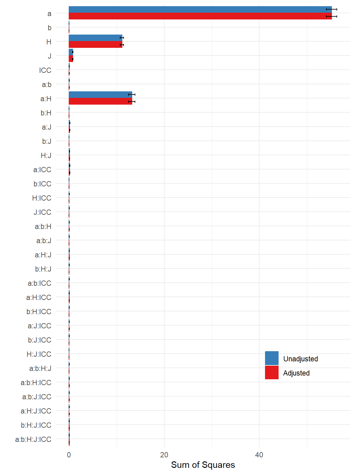
@fig-SS-adjusted visualizes the original (unadjusted) and adjusted sums of squares for each term.
It's clear that the adjustment does not change the story at all: there's still three big terms ($a$, $H$, and $a:H$) plus one smaller one ($J$) and the rest are trivial.
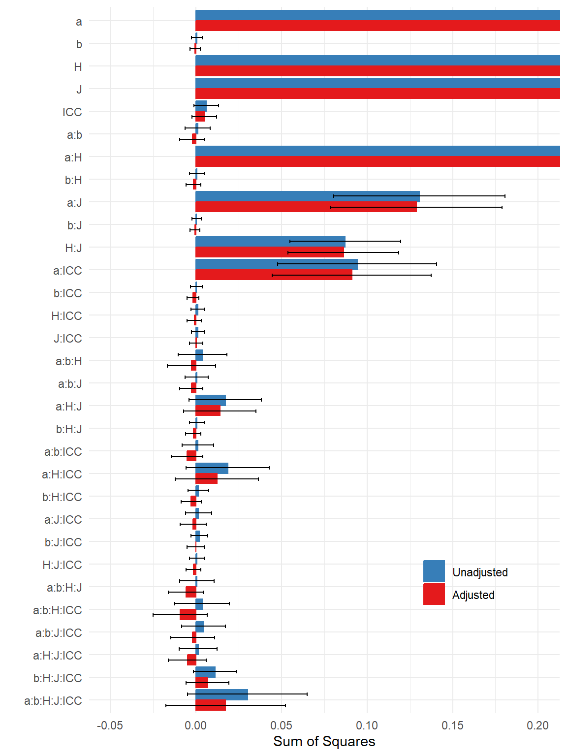
Click on the "ZOOMED IN" tab to see @fig-SS-adjusted-zoom, which makes it easier to see the difference between the unadjusted and adjusted sums of squares for the trivial terms.
It can be seen that the adjustment term sometimes makes the sum of squares negative.
The underlying data are in @tbl-Lee-SS-adjusted in the "DATA" tab.
::: {.panel-tabset}
### Zoomed out
```{r}
#| label: fig-SS-adjusted
#| fig-cap: Unadjusted and adjusted sums of squares for Root Mean Squared Error of the CCREM estimator
#| fig-width: 6
#| fig-height: 8
#| echo: false
SS_long <-
SS_adjusted_full %>%
select(-A, -df) %>%
pivot_longer(c(SS, SSA), names_to = "type", values_to = "SS") %>%
mutate(
term = factor(term, levels = rev(unique(term))),
type = recode_values(type, "SS" ~ "Unadjusted", "SSA" ~ "Adjusted"),
SS_l = SS - qnorm(.975) * SSA_mcse,
SS_u = SS + qnorm(.975) * SSA_mcse
)
p <-
ggplot(SS_long) +
aes(SS, term, color = type, fill = type) +
geom_col(position = "dodge") +
geom_errorbar(
aes(xmin = SS_l, xmax = SS_u),
position = position_dodge(width = 1),
width = 0.3,
color = "black"
) +
theme_minimal() +
scale_fill_brewer(
type = "qual", palette = 6,
guide = guide_legend(reverse = TRUE),
aesthetics = c("color","fill")
) +
labs(x = "Sum of Squares", y = "", color = "", fill = "") +
theme(legend.position = "inside", legend.position.inside = c(0.8,0.2))
p
```
### Zoomed in
```{r}
#| label: fig-SS-adjusted-zoom
#| fig-cap: Unadjusted and adjusted sums of squares for Root Mean Squared Error of the CCREM estimator (zoomed in)
#| fig-width: 6
#| fig-height: 8
#| echo: false
p + coord_cartesian(xlim = c(-0.05,0.20))
```
### Data
```{r}
#| echo: false
#| label: tbl-Lee-SS-adjusted
#| tbl-cap: Adjusted sums of squares for Root Mean Squared Error of the CCREM estimator, based on a fully saturated model
SS_adjusted_full %>%
rename(`Sum Sq` = SS, Df = df, Adj = A, `Sum Sq Adj` = SSA, MCSE = SSA_mcse) %>%
tt() %>%
format_tt(digits = 4, num_fmt = "decimal") %>%
style_tt(j = 2:5, align = "r") %>%
theme_striped()
```
:::
Here's how to apply the function to compute the adjusted ANOVA for RMSE from @lee2024comparing, but using a greatly simplified model and computing p-values for null hypothesis tests on each component:
```{r}
#| code-fold: show
SS_adjusted_reduced <- meta_aov(
  rmse ~ a + H + J + a:H + a:J + H:J,
  mcse = rmse_mcse,
  data = CCREM_res,
  test = TRUE
)
```
@tbl-Lee-SS-adjusted-reduced reports the resulting ANOVA table, which includes the result of testing the null that the residual variation is zero. The p-value is very large, indicating that the data are consistent with the possibility that the reduced model is sufficient to explain all of the true variation in the performance measure.
It's a bit curious that the Satterthwaite degrees of freedom (labeled as 'nu') for each of the included terms are so small, but this might be because there's substantial heteroskedasticity in the Monte Carlo error.
```{r}
#| echo: false
#| label: tbl-Lee-SS-adjusted-reduced
#| tbl-cap: Adjusted sums of squares for Root Mean Squared Error of the CCREM estimator, based on a reduced model
SS_adjusted_reduced %>%
mutate(
pval = format.pval(pval, eps = 1e-3, nsmall = 3, justify = "right")
) %>%
rename(`Sum Sq` = SS, Df = df, Adj = A, `Sum Sq Adj` = SSA, MCSE = SSA_mcse, `p-value` = pval) %>%
tt() %>%
format_tt(j = 3:6, digits = 4, num_fmt = "decimal", num_zero = TRUE) %>%
format_tt(j = 7:8, digits = 2, num_fmt = "decimal", num_zero = TRUE) %>%
style_tt(j = 2:9, align = "r") %>%
theme_striped()
```
## Remarks
I have never seen this sort of analysis conducted on Monte Carlo simulation results.
Based on this example, it strikes me as something that might be worth developing further.
Of course, I should probably temper my enthusiasm considering how small the adjustments are relative to the magnitude of the sums of squares involved.
In practice, it's probably fine to just focus on the magnitude of the raw sums of squares.
But it does seem helpful to be able to gauge the magnitude of the Monte Carlo standard errors on the sums of squares.
And it also seems like this sort of analysis could be useful in supporting an argument that some of the factors in a design can safely be ignored (or averaged over).
I'm going to keep playing with these ideas to see where they go.
If you found any of this remotely interesting, or if you try out the `meta_aov()` function and find something interesting, perplexing, or confusing in the output, please feel free to reach out.