---
title: Copas selection models for meta-analysis
date: '2024-07-27'
categories:
- effect size
- distribution theory
- selective reporting
execute:
echo: false
bibliography: "../selection-references.bib"
csl: "../apa.csl"
link-citations: true
code-tools: true
toc: true
css: styles.css
crossref:
eq-prefix: ""
---
Recently, I've been studying and tinkering with meta-analytic models for selective reporting of findings from primary studies.
I've mostly focused on [step-function selection models](/posts/step-function-selection-models/) [@hedges1992modeling; @vevea1995general; @Hedges1996estimating; @vevea2005publication], which assume that selective reporting of primary study results is driven by the $p$-values of the effect size estimates (and specifically, where those $p$-values fall relative to certain thresholds).
This is not the only form of selection model, though.
One prominent alternative model, described in a series of papers by John Copas and colleagues [@copas1997inference; @copas1999what; @copas2000metaanalysis; @Copas2001sensitivity], is based on distinctly different assumptions than the step-function model.
The Copas selection model has received a fair amount of attention in the literature on meta-analysis of medical and epidemiological research, but relatively little attention from the social science side of things.
In this post, I'll give an overview of the Copas model and try to highlight some of the ways that it differs from step function selection models.
# The Copas selection model
Similar to the step function selection model, the Copas model is composed of two components: an _evidence-generating process_ that describes the distribution of effect size estimates prior to selection and a _selective reporting process_ that describes how selective reporting happens as a function of the effect size estimates and associated quantities like standard errors and $p$-values.
The evidence-generating process is just a conventional random effects model.
Letting $T_i^*$ denote an effect size estimate prior to selective reporting, $\theta_i^*$ denote the corresponding effect size parameter, and $\sigma_i^*$ denote its (known) standard error, we assume that effect size estimate $i$ is drawn from a normal distribution with mean $\theta_i^*$ and standard deviation $\sigma_i^*$:
$$
T_i^* | \theta_i^*, \sigma_i^* \sim N\left(\theta_i^*, \left(\sigma_i^*\right)^2\right).
$$ {#eq-evidence-generation-level1}
We further assume that the effect size parameters are drawn from a normal distribution with overall average effect size $\mu$ and standard deviation $\tau$:
$$
\theta_i^* | \sigma_i^* \sim N\left(\mu, \tau^2\right).
$$ {#eq-evidence-generation-level2}
The full evidence-generating process can also be written as a random effects model with two sources of error:
$$
T_i^* = \mu + \nu_i^* + \epsilon_i^*,
$$ {#eq-evidence-generation-full}
where $\nu_i^* \sim N(0, \tau^2)$ and $\epsilon_i^* \sim N\left(0, \left(\sigma_i^*\right)^2\right)$.
The second component is where the Copas model diverges from the step-function model. The Copas model posits that selection is driven by a latent index $\zeta_i$ that is normally distributed and correlated with $\epsilon_i^*$, with mean that is a function of $\sigma_i^*$:
$$
\zeta_i = \alpha + \frac{\beta}{\sigma_i^*} + \delta_i,
$$ {#eq-selection}
where $\delta_i \sim N(0, 1)$ and $\text{cor}(\delta_i, \epsilon_i^*) = \rho$.
With this specification, $T_i^*$ is reported (and thus available for inclusion in a meta-analysis) if $\zeta_i > 0$ and is otherwise unreported.
Following the notation of my previous post, I'll use $O_i^*$ to denote a binary indicator equal to 1 if $T_i^*$ is reported and otherwise equal to zero. With this notation, $\Pr\left(O_i^* = 1 | \sigma_i^*\right) = \Pr\left(\zeta_i > 0 | \sigma_i^*\right)$.
@Copas2001sensitivity calls $\zeta_i$ the _propensity for selection_.
Under the posited model, the selection propensity depends both on the precision of the study through $\sigma_i^*$ (because the mean of $\zeta_i$ depends on the inverse of $\sigma_i^*$) and on the magnitude of the reported effect size estimate (because $\zeta_i$ is correlated with $\epsilon_i^*$).
The parameter $\alpha$ controls the overall probability of selection, irrespective of the findings; $\beta$ controls how strongly selection depends on study precision; and $\rho$ controls how strongly selection depends on the magnitude of the effect size estimate itself.
The Copas model posits a stable correlation $\rho$ between the selection propensity index and the _samplng error_ of the random effects model, $\epsilon_i^*$.
If there is heterogeneity in the effect size parameters and heterogeneity in the sampling variances, then the correlation between $\zeta_i$ and $T_i^*$ will be lower than $\rho$ and will differ from study to study.
With a little variance algebra, it can be seen that
$$
\text{cor}\left(\zeta_i, T_i^* | \sigma_i^*\right) = \tilde\rho_i = \frac{\rho \sigma_i^*}{\sqrt{\tau^2 + \left(\sigma_i^*\right)^2}}.
$$ {#eq-zeta-correlation}
Using the correlation, we can write the selection propensity index in terms of a regression on $T_i^*$:
$$
\zeta_i | T_i^*, \sigma_i^* \sim N \left(\alpha + \frac{\beta}{\sigma_i^*} + \tilde\rho_i \left(\frac{T_i^* - \mu}{\sqrt{\tau^2 + \left(\sigma_i^*\right)^2}}\right), \ 1 - \rho_i^2\right).
$$
Thus, given the effect size estimate $T_i^*$ and its standard error $\sigma_i^*$, the probability that finding $i$ is reported is
$$
\Pr\left(O_i^* = 1 | T_i^*, \sigma_i^*\right) = \Phi\left(\frac{1}{\sqrt{1 - \tilde\rho_i^2}}\left[\alpha + \frac{\beta}{\sigma_i^*} + \tilde\rho_i \left(\frac{T_i^* - \mu}{\sqrt{\tau^2 + \left(\sigma_i^*\right)^2}}\right)\right]\right)
$$ {#eq-conditional-selection-probability}
[@Copas2001sensitivity, Equation 4; @hedges2005selection, Equation 9.6].
# Distribution of observed effect sizes
The observed effect size estimates $T_i$ follow a distribution equivalent to that of $\left(T_i^* | \sigma_i^*, O_i^* = 1\right)$. It's possible to find an analytic expression for the density of the observed effect sizes. Using Bayes Theorem, the density of the observed $T_i$'s is
$$
\Pr\left(T_i = t| \sigma_i^*\right) = \Pr\left(T_i^* = t | \sigma_i^*, O_i^* = 1\right) = \frac{\Pr\left(O_i^* = 1 | T_i^* = t, \sigma_i^*\right) \times \Pr\left(T_i^* = t | \sigma_i^*\right)}{\Pr\left(O_i^* = 1 | \sigma_i^*\right)},
$$ {#eq-Bayes-theorem}
where the first term in the numerator is given in (@eq-conditional-selection-probability), the second term in the numerator can be derived from (@eq-evidence-generation-full), and the denominator can be derived from (@eq-selection).
Letting $\eta_i = \sqrt{\tau^2 + \left(\sigma_i^*\right)^2}$ and substituting everything into the above gives
$$
\Pr\left(T_i = t| \sigma_i^*\right) = \frac{1}{\eta_i} \phi\left(\frac{t - \mu}{\eta_i}\right) \times \frac{\Phi\left(\frac{1}{\sqrt{1 - \tilde\rho_i^2}}\left[\alpha + \frac{\beta}{\sigma_i^*} + \tilde\rho_i \left(\frac{t - \mu}{\eta_i}\right)\right]\right)} {\Phi\left(\alpha + \frac{\beta}{\sigma_i^*}\right)}.
$$ {#eq-observed-density}
This density is identical to that of the _generalized skew-normal distribution_ [@arellano20006unification].
Here is an interactive graph showing the distribution of the effects prior to selection (in grey) and the distribution of observed effect sizes (in blue) based on the Copas selection model.[^unnormalized]
Initially, the selection parameters are set to $\alpha = -3$, $\beta = 0.5$ and $\rho = 0.5$, but you can change these however you like. Try wiggling $\rho$ up and down to see how the bias and shape of the density changes.
[^unnormalized]: Note that I've plotted the _unnormalized density_ (the density before dividing by $\Phi\left(\alpha + \frac{\beta}{\sigma_i^*}\right)$) so that it's clear that the distribution of observed effects is a subset of the distribution of effects prior to selection.
```{ojs}
math = require("mathjs")
norm = import('https://unpkg.com/norm-dist@3.1.0/index.js?module')

eta = math.sqrt(tau**2 + sigma**2)
rho_i = rho * sigma / eta
u = alpha + beta / sigma
lambda = norm.pdf(u) / norm.cdf(u)

Ai = norm.cdf(u)
ET = mu + rho * sigma * lambda
SDT = eta * math.sqrt(1 - rho_i**2 * lambda * (u + lambda))
Ai_toprint = Ai.toFixed(3)
ET_toprint = ET.toFixed(3)
eta_toprint = eta.toFixed(3)
SDT_toprint = SDT.toFixed(3)

function CopasSelection(t, s, alpha, beta, rho) {
  let u = alpha + beta / s;
  let eta_ = math.sqrt(tau**2 + s**2);
  let rho_i_ = rho * s / eta_;
  let z = (t - mu) / eta_;
  let x = (u + rho_i_ * z) / math.sqrt(1 - rho_i_**2);
  return norm.cdf(x);
}
```
```{ojs}
pts = 201

dat = Array(pts).fill().map((element, index) => {
  let t = mu - 3 * eta + index * eta * 6 / (pts - 1);
  let dt = norm.pdf((t - mu) / eta) / eta;
  let pr_sel = CopasSelection(t, sigma, alpha, beta, rho);
  return ({
    t: t,
    d_unselected: dt,
    d_selected: pr_sel * dt
  })
})
```
::::: {.grid .column-page}
:::: {.g-col-8 .center}
```{ojs}
Plot.plot({
  height: 300,
  width: 700,
  y: {
    grid: false,
    label: "Density"
  },
  x: {
    label: "Effect size estimate (Ti)"
  },
  marks: [
    Plot.ruleY([0]),
    Plot.ruleX([0]),
    Plot.areaY(dat, {x: "t", y: "d_unselected", fillOpacity: 0.3}),
    Plot.areaY(dat, {x: "t", y: "d_selected", fill: "blue", fillOpacity: 0.5}),
    Plot.lineY(dat, {x: "t", y: "d_selected", stroke: "blue"})
  ]
})
```
:::{.moments}
```{ojs}
tex`
\begin{aligned}
\mu &= ${mu} & \qquad \eta_i &= ${eta_toprint} \\
\mathbb{E}\left(T_i | \sigma_i\right) &= ${ET_toprint}
& \qquad \sqrt{\mathbb{V}\left(T_i | \sigma_i\right)} &= ${SDT_toprint} \\
\Pr(O_i^* = 1 | \sigma_i^*) &= ${Ai_toprint}
\end{aligned}
`
```
:::
::::
:::: {.g-col-4}
```{ojs}
//| panel: input
viewof mu = Inputs.range(
  [-2, 2],
  {value: 0.15, step: 0.01, label: tex`\mu`}
)

viewof tau = Inputs.range(
  [0, 2],
  {value: 0.10, step: 0.01, label: tex`\tau`}
)

viewof sigma = Inputs.range(
  [0, 1],
  {value: 0.20, step: 0.01, label: tex`\sigma_i`}
)

viewof alpha = Inputs.range(
  [-10, 10],
  {value: -3, step: 0.1, label: tex`\alpha`}
)

viewof beta = Inputs.range(
  [0, 2],
  {value: 0.5, step: 0.01, label: tex`\beta`}
)

viewof rho = Inputs.range(
  [-1, 1],
  {value: 0.5, step: 0.01, label: tex`\rho`}
)
```
::::
:::::
# Moments of $T_i | \sigma_i$
@arnold1999nontruncated derived the moment-generating function and first several moments of a further generalization of the skew-normal distribution, of which the distribution of $T_i$ is a special case. Letting $Z_i = \frac{T_i - \mu}{\sqrt{\tau^2 + \sigma_i^2}}$, $u_i = \alpha + \frac{\beta}{\sigma_i}$, and $\lambda(u_i) = \phi(u_i) / \Phi(u_i)$, they give the first two moments of $Z_i$ as
$$
\begin{aligned}
\mathbb{E}\left(Z_i | \sigma_i \right) &= \rho_i \lambda\left(u_i\right) \\
\mathbb{E}\left(Z_i^2 | \sigma_i \right) &= 1 - \rho_i^2 u_i \lambda(u_i)
\end{aligned}
$$
by which it follows that
$$
\begin{aligned}
\mathbb{E}\left(T_i | \sigma_i \right) &= \mu + \sqrt{\tau^2 + \sigma_i^2} \times \rho_i \lambda\left(u_i\right) \\
&= \mu + \rho \sigma_i \lambda\left(u_i\right)
\end{aligned}
$$ {#eq-Ti-mean}
and
$$
\begin{aligned}
\mathbb{V}\left(T_i | \sigma_i \right) &= \left(\tau^2 + \sigma_i^2\right) \left(1 - \rho_i^2\lambda(u_i) \times [u_i + \lambda(u_i)]\right) \\
&= \tau^2 + \sigma_i^2\left(1 - \rho^2 \lambda(u_i) \times [u_i + \lambda(u_i)]\right).
\end{aligned}
$$ {#eq-Ti-variance}
The expression for $\mathbb{E}\left(T_i | \sigma_i \right)$ is also given in @copas2000metaanalysis and @Copas2001sensitivity.[^variance-of-T]
[^variance-of-T]: These sources give the variance of the observed effect size estimates as $\mathbb{V}\left(T_i | \sigma_i \right) = \sigma_i^2\left(1 - \rho^2 \lambda(u_i) \times [u_i + \lambda(u_i)]\right)$ [see p. 250 of @copas2000metaanalysis; see Equation 6 of @Copas2001sensitivity]. However, these expressions are incorrect as stated because they omit the between-study heterogeneity $\tau^2$.
Several things are noteworthy about these expressions.
For one, the expectation of $T_i$ is additive in $\mu$, so the bias $\mathbb{E}(T_i | \sigma_i) - \mu$ does not depend on the location of the distribution prior to selection. Nor does it depend on the degree of heterogeneity $\tau$.
Likewise, the variance of $T_i$ is additive in $\tau^2$. Only the sampling variance is affected by selection.
All of these properties are in contrast to the step-function selection model, where both the bias and the variance are complex functions that _do_ depend on $\mu$ and $\tau$.
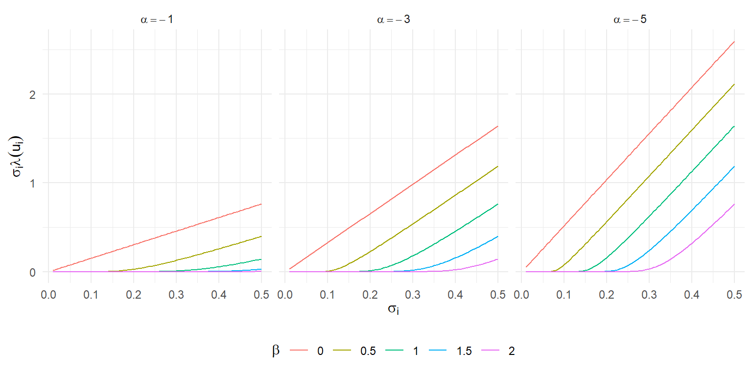
Under the Copas model, the bias of $T_i$ is directly proportional to $\rho$ and is a more complicated function of $\alpha$ and $\beta$ (through $u_i$).
The bias is an increasing function of $\sigma$, the shape of which depends on $\alpha$ and $\beta$.
Here's an illustration of $\sigma_i \times \lambda(u_i)$ as a function of $\sigma_i$ for a few different values of the selection parameters:
```{r}
#| fig-width: 8
#| fig-height: 4
#| out-width: 100%
#| fig-retina: 2
library(tidyverse)
df <- expand_grid(
sigma = seq(0.01, 0.50, 0.005),
alpha = c(-1, -3, -5),
beta = seq(0, 2, 0.5)
) %>%
mutate(
u = alpha + beta / sigma,
lambda = dnorm(u) / pnorm(u),
bias = sigma * lambda,
beta_f = factor(beta),
alpha_f = paste0("alpha ==", alpha)
)
ggplot(df, aes(sigma, bias, color = beta_f)) +
facet_wrap(~ alpha_f, labeller = label_parsed) +
geom_line() +
theme_minimal() +
theme(legend.position = "bottom") +
labs(
x = expression(sigma[i]),
y = expression(sigma[i] * lambda(u[i])),
color = expression(beta)
)
```
When $\beta = 0$, the bias is directly proportional to $\sigma_i$, just like in an Egger regression or the PET meta-regression adjustment method [@stanley2008metaregression].
As $\beta$ increases, the bias is initially very close to zero and then grows almost linearly after a certain point---much as in the kinked meta-regression adjustment proposed by @bom2019kinked.
Very curious.
# Funnel density
Here is an interactive funnel plot showing the distribution of effect size estimates under the Copas selection model. I initially set $\mu = 0.15$ and $\tau = 0.10$ and selection parameters of $\alpha = -3$, $\beta = 0.5$ and $\rho = 0.5$, but you can change these however you like.
```{ojs}
SE_pts = 100
t_pts = 181
sigma_max = 0.5
eta_max_f = math.sqrt(tau_f**2 + sigma_max**2)

funnel_dat = Array(t_pts * SE_pts).fill(null).map((x,row) => {
  let i = row % SE_pts;
  let j = (row - i) / SE_pts;
  let sigma = (i + 1) * sigma_max / SE_pts;
  let t = mu_f - 3 * eta_max_f + j * eta_max_f * 6 / (t_pts - 1);
  let eta = math.sqrt(tau_f**2 + sigma**2);
  let dt = norm.pdf((t - mu_f) / eta) / eta;
  let pr_sel = CopasSelection(t, sigma, alpha_f, beta_f, rho_f);
  return ({t: t, sigma: sigma, dt: dt, pr_sel: pr_sel, d_selected: pr_sel * dt});
})

sigline_dat = [
  ({t: 0, sigma: 0}),
  ({t: sigma_max * norm.icdf(0.975), sigma: sigma_max})
]
```
::::: {.grid .column-page}
:::: {.g-col-8 .center}
```{ojs}
Plot.plot({
  height: 400,
  width: 700,
  padding: 0,
  grid: false,
  x: {axis: "top", label: "Effect size estimate (Ti)"},
  y: {label: "Standard error (sigma_i)", reverse: true},
  color: {
    scheme: "pubugn",
    type: "sqrt",
    label: "Density"
  },
  marks: [
    Plot.dot(funnel_dat, {x: "t", y: "sigma", fill: "d_selected", r:2, symbol: "square"}),
    Plot.ruleY([0], {stroke: "black"}),
    Plot.ruleX([0], {stroke: "grey"}),
    Plot.line(sigline_dat, {x: "t", y: "sigma", stroke: "gray", strokeWidth: 1})
  ]
})
```
```{ojs}
Plot.legend({color: {scheme: "pubugn", type: "sqrt", label: "Density"}})
```
::::
:::: {.g-col-4}
```{ojs}
//| panel: input
viewof mu_f = Inputs.range(
  [-2, 2],
  {value: 0.15, step: 0.01, label: tex`\mu`}
)

viewof tau_f = Inputs.range(
  [0, 2],
  {value: 0.10, step: 0.01, label: tex`\tau`}
)

viewof alpha_f = Inputs.range(
  [-10, 10],
  {value: -3, step: 0.1, label: tex`\alpha`}
)

viewof beta_f = Inputs.range(
  [0, 2],
  {value: 0.5, step: 0.01, label: tex`\beta`}
)

viewof rho_f = Inputs.range(
  [-1, 1],
  {value: 0.5, step: 0.01, label: tex`\rho`}
)
```
::::
:::::
The funnel plot shows the _un-normalized_ distribution of the observed effect sizes conditional on $\sigma_i$. One of the very striking things about the funnel is just how steeply the marginal selection probabilities (i.e., $\Pr(O_i^* = 1| \sigma_i^*)$) drop off as $\sigma_i$ increases (going from the top to the bottom of the plot).
With the initial parameter settings, findings from small studies with large $\sigma_i$s are generally _quite_ unlikely to be published, regardless of their significance or effect size.
Increasing $\alpha$ will increase the marginal selection probability for all studies, though in a non-linear way depending on their $\sigma_i$'s.
Reducing $\beta$ will mitigate the drop-off in selection probabilities from large studies to small ones.
# Comments
There are several aspects of the Copas model that I find somewhat perplexing.
One is the assumption that the selection propensity index is correlated with the _sampling errors_ rather than with the marginal distribution of $T_i^*$.
Taken literally, this means that the selection propensity depends not just on the effect size estimate (which is an observable quantity) but on where that estimate lies relative to the true study-specific effect size parameter $\theta_i$.
It seems more plausible to me that authors, reviewers, editors, etc. would make decisions that could influence selective reporting based on observable quantities such as effect size estimates, standard errors, or $p$-values (as in the [step-function selection model](/posts/step-function-selection-models/)).
Another perplexing aspect of the model is that, for a given set of selection parameters $\alpha$, $\beta$, and $\rho$, the bias due to selection is constant and unaffected by the location $\mu$ or scale $\tau$ of the true effect size distribution.
As a result, under the model's posited form of selection bias, the extent of bias is disconnected from considerations of statistical significance or power.
In practice, I would expect the risk of selection bias to be greater for small studies examining small effects than for small studies examining very strong effect sizes, but the parameterization of the Copas model makes it kind of hard to capture such a pattern.
Put another way, I think this implies that the plausibility of a given selection parameters $\alpha$, $\beta$, and $\rho$ might actually depend on $\mu$ and $\tau$.
Third, a well known aspect of the model is that its three selection-related parameters are only very weakly identifiable from observed effect size distributions.
Because of this, the Copas model is typically used as a sort of sensitivity analysis, where the analyst estimates $\mu$, $\tau$, and $\rho$ by maximum likelihood [@Copas2001sensitivity] for specified values for $\alpha$ and $\beta$, and then examines how these parameter estimates vary across a range of possible $\alpha$ and $\beta$.[^empirical-priors]
But sensitivity analysis is only really helpful to the extent that the analyst can specify a plausible range of values for the selection parameters, which is hard to do if the plausible range depends on $\mu$ and $\tau$.
Other scholars have proposed using the Copas in a Bayesian framework [e.g., @bai2021robust; @mavridis2013fully], but it seems like similar concerns would apply---if key parameters are only weakly identified, then their priors may be strongly influential, but if it's hard to formulas credible priors....
[^empirical-priors]: Some recent work by @huang2021using proposes using clinical trial registry information to estimate all the parameters of the Copas model, which seems like an interesting and potentially useful strategy.
To be clear, my comments here are all just half-baked impressions as I work through a model that's pretty new to me.
Copas has some more recent work that considers alternative assumptions about the selective reporting process [@copas2013likelihood], which seem simpler and more closely connected to $p$-value-based selection processes.
However, other scholars have continued to study and extend the Copas selection model [e.g., @duan2020testing; @ning2017maximum; @piao2019copas], so I probably just need to read more about how it's applied to get a better sense of its strengths and utility.
Comments
There are several aspects of the Copas model that I find somewhat perplexing. One is the assumption that the selection propensity index is correlated with the sampling errors rather than with the marginal distribution of \(T_i^*\). Taken literally, this means that the selection propensity depends not just on the effect size estimate (which is an observable quantity) but on where that estimate lies relative to the true study-specific effect size parameter \(\theta_i\). It seems more plausible to me that authors, reviewers, editors, etc. would make decisions that could influence selective reporting based on observable quantities such as effect size estimates, standard errors, or \(p\)-values (as in the step-function selection model).
Another perplexing aspect of the model is that, for a given set of selection parameters \(\alpha\), \(\beta\), and \(\rho\), the bias due to selection is constant and unaffected by the location \(\mu\) or scale \(\tau\) of the true effect size distribution. As a result, under the model’s posited form of selection bias, the extent of bias is disconnected from considerations of statistical significance or power. In practice, I would expect the risk of selection bias to be greater for small studies examining small effects than for small studies examining very strong effect sizes, but the parameterization of the Copas model makes it kind of hard to capture such a pattern. Put another way, I think this implies that the plausibility of a given selection parameters \(\alpha\), \(\beta\), and \(\rho\) might actually depend on \(\mu\) and \(\tau\).
Third, a well known aspect of the model is that its three selection-related parameters are only very weakly identifiable from observed effect size distributions. Because of this, the Copas model is typically used as a sort of sensitivity analysis, where the analyst estimates \(\mu\), \(\tau\), and \(\rho\) by maximum likelihood (Copas & Shi, 2001) for specified values for \(\alpha\) and \(\beta\), and then examines how these parameter estimates vary across a range of possible \(\alpha\) and \(\beta\).3 But sensitivity analysis is only really helpful to the extent that the analyst can specify a plausible range of values for the selection parameters, which is hard to do if the plausible range depends on \(\mu\) and \(\tau\). Other scholars have proposed using the Copas in a Bayesian framework (e.g., Bai et al., 2021; Mavridis et al., 2013), but it seems like similar concerns would apply—if key parameters are only weakly identified, then their priors may be strongly influential, but if it’s hard to formulas credible priors….
To be clear, my comments here are all just half-baked impressions as I work through a model that’s pretty new to me. Copas has some more recent work that considers alternative assumptions about the selective reporting process (Copas, 2013), which seem simpler and more closely connected to \(p\)-value-based selection processes. However, other scholars have continued to study and extend the Copas selection model (e.g., Duan et al., 2020; Ning et al., 2017; Piao et al., 2019), so I probably just need to read more about how it’s applied to get a better sense of its strengths and utility.