Code
set.seed(20240629)
N <- 50
mu <- 2
nu <- 5
dat <- mu + rt(N, df = nu)Bootstrapping is a brilliant statistical idea. I realize that it’s become pretty routine, these days, and maybe has lost some of the magical veneer it once had, but I will fess up that I am still a fanboy. I teach my students to think of bootstrapping as your back-pocket tool for inference: if you’re not sure how to get a standard error or a confidence interval for some quantity that you’ve estimated, bootstrapping is probably a good place to start—and possibly good enough.
The core idea behind bootstrap inference is to use simulation to emulate the process of collecting a sample, and to take the variation across simulation results as a proxy for the sampling uncertainty in your real data. A sample of \(B\) simulated results (which we might call booties) form the basis of bootstrap standard errors, confidence intervals, hypothesis tests, and the like. The simulation process can be as simple as re-sampling observations from your original data, in which case the original sample is a stand-in for the population and each re-sample is a replication of the process of collecting a dataset for analysis. Other simulation processes are possible too, which can account for more complex study designs or make stronger use of parametric modeling assumptions.
Across all its variations, bootstrapping involves using brute-force computation to do something that would otherwise take a bunch of math (like delta-method calculations). This same feature makes it a royal pain to study bootstrap techniques using Monte Carlo simulation. In a Monte Carlo simulation, one has to generate hypothetical data, apply an estimator to each simulated dataset, and then repeat the whole process \(R\) times (for some large \(R\)) to see the sampling distribution of the estimator. But if the estimator itself requires doing a bunch of re-sampling (or some other form of simulation) just to get one confidence interval, then the computation involved in the whole process can be pretty demanding. In this post, I’ll look at a trick that can make the whole process a bit more efficient.
Boos & Zhang (2000) proposed a technique for approximating the power of a \(B = \infty\) bootstrap test, while using only a finite, feasibly small number of replicates. Their work focused on hypothesis tests, but the approach applies directly to confidence interval simulations as well. The trick is to calculate the bootstrap test several times for each replication, each time with a different number of booties, and then extrapolate to \(B = \infty\).
Suppose we’re doing a simulation to evaluate the properties of a some sort of bootstrap confidence interval, where the main performance characteristics of interest are the coverage rate and the average width of the intervals. The simulation process will need to be repeated \(R\) times, and \(R\) will need to be fairly large to control the Monte Carlo error in the simulation results (e.g., to ensure that Monte Carlo standard errors for coverage rates will be less than 1%, we’ll need to run at least 2500 replications). For each of those replications, we’ll need to do \(B\) bootstrap replications (ahem, booties!) to obtain a confidence interval. On top of all that, we will also often want to repeat the whole process across a number of different conditions. For example, the first simulation in Joshi et al. (2022) involved a \(4 \times 2 \times 2 \times 11\) factorial design (176 total conditions), with \(R = 2400\) replications per condition and \(B = 399\) booties per replication. It quickly adds up—or rather, it quickly multiplies out!
A challenge here is that the power of a bootstrap hypothesis test depends on \(B\) (as discussed in Davidson & MacKinnon, 2000); by extension, so too does the coverage rate and width of a bootstrap confidence interval. If we use only a small number of booties, then the simulation results will under-state coverage relative to what we might obtain when applying the method in practice (where we might use something more like \(B = 1999\) or \(3999\)) But if we use a realistically large number of booties, then our simulations will take forever to finish…or we’ll have to cut down on the number of conditions include…or both…or maybe we’ll decide that the delta-method math isn’t so bad after all.
Now imagine that we generate \(B\) booties, but then take several simple random sub-samples from the booties, of size \(B_1 < B_2 <... < B_P = B\). Each of these is a valid bootstrap sample, but using a smaller number of booties. We can calculate a confidence interval for each one, so we end up with a total of \(P \times R\) confidence intervals. Let \(C_{br}\) be an indicator for whether replication \(r\) of the confidence interval with \(b\) booties covers the true parameter, for \(b = B_1,B_2,...,B_P\) and \(r = 1,...,R\). We can extrapolate the coverage rate using a linear regression1 of \(C_{br}\) on \(1 / b\): \[ C_{br} = \alpha_0 + \alpha_1 \frac{1}{b} + \epsilon_{br}. \] Then \(\alpha_0\) is the coverage rate when \(b = \infty\). The outcomes \(C_{B_1r},...,C_{B_P r}\) will be dependent because they’re based on the same set of booties. However, the replicates are independent, so we can just use cluster-robust variance estimators to get Monte Carlo standard errors for an estimate of \(\alpha_0\). Essentially the same thing works for extrapolating the width of a \(B = \infty\) confidence interval: just replace \(C_{br}\) with \(W_{br}\), the width of the confidence interval based on the \(b^{th}\) bootstrap subsample from replication \(r\).
In the context of hypothesis testing problems, Boos & Zhang (2000) actually proposed something a little bit more complicated than what I’ve described above. Instead of just taking a single sub-sample of each size \(B_1,...,B_P\), they note that that expected rejection rate for each size sub-sample can be computed using hypergeometric probabilities. The same thing works for computing confidence interval coverage, but I don’t see any way to make it work for confidence interval width. However, instead of computing just one sub-sample of size \(b\), we could compute several and then average across them to approximate the expected value of \(C_{br}\) or \(W_{br}\) given the full set of \(B\) booties.
Here’s an example of how this all works. For sake of simplicity (and compute time), I’m going to use an overly simple, not particularly well-motivated example of bootstrapping: using a percentile bootstrap for the population mean, where the estimator is a trimmed sample mean. As a data-generating process, I’ll use a shifted \(t\) distribution with population mean \(\mu\) and degrees of freedom \(\nu\): \[ Y_1,...,Y_N \stackrel{iid}{\sim} \mu + t(\nu) \] Or in R code:
set.seed(20240629)
N <- 50
mu <- 2
nu <- 5
dat <- mu + rt(N, df = nu)As an estimator, I’ll use the 10% trimmed mean:
y_bar_trim <- mean(dat, trim = 0.1)A bootstrap confidence interval for \(\mu\) can be computed as follows:
B <- 399
booties <- replicate(B, {
  sample(dat, size = N, replace = TRUE) |>
  mean(trim = 0.1)
})
quantile(booties, c(.025, .975))
2.5% 97.5%
1.491885 2.255334 Now, instead of computing just the one CI based on all \(B\) booties, I’ll also compute confidence intervals for several smaller subsamples from the booties:
library(tidyverse)

B_vals <- c(39, 59, 79, 99, 199, 399) # sub-sample sizes
m <- 10 # number of CIs per B_val

sub_boots <- map(B_vals, \(x) {
  if (x == length(booties)) m <- 1L
  replicate(m , {
    sample(booties, size = x, replace = TRUE) |>
    quantile(c(.025, .975))
  }, simplify = FALSE)
})
The result in sub_boots is a list with one entry per sub-sample size, where each entry includes \(m = 10\) bootstrap confidence intervals.
Now I’ll compute the expected coverage rate and interval width for each of the B_vals:
boot_coverage <- map_dbl(sub_boots, \(x) {
  map_dbl(x, \(y) y[1] < mu & mu < y[2]) |>
    mean()
})
boot_width <- map_dbl(sub_boots, \(x) {
  map_dbl(x, diff) |>
    mean()
})
boot_performance <- data.frame(
  B = B_vals,
  coverage = boot_coverage,
  width = boot_width
)
boot_performance
B coverage width
1 39 1 0.7400180
2 59 1 0.7680832
3 79 1 0.7214260
4 99 1 0.7424530
5 199 1 0.7519438
6 399 1 0.7809795The above is just for a single realization of the data-generating process, so it’s not particularly revealing. More interesting is if we replicate the whole process a bunch of times:
dgp <- function(N, mu, nu) {
  mu + rt(N, df = nu)
}

estimator <- function(
    dat, # data
    B_vals = 399, # number of booties to evaluate
    m = 1, # CIs to replicate per sub-sample size
    trim = 0.1 # trimming percentage
  ) {

  # compute booties
  N <- length(dat)
  booties <- replicate(max(B_vals), {
    sample(dat, size = N, replace = TRUE) |>
    mean(trim = 0.1)
  })

  # confidence intervals for each B_vals
  sub_boots <- map(B_vals, \(x) {
    if (x == length(booties)) m <- 1L
    replicate(m , {
      sample(booties, size = x, replace = TRUE) |>
      quantile(c(.025, .975))
    }, simplify = FALSE)
  })

  # coverage rates
  boot_coverage <- map_dbl(sub_boots, \(x) {
    map_dbl(x, \(y) y[1] < mu & mu < y[2]) |>
      mean()
  })

  # CI widths
  boot_width <- map_dbl(sub_boots, \(x) {
    map_dbl(x, diff) |>
      mean()
  })

  # put it all together
  data.frame(
    B = B_vals,
    coverage = boot_coverage,
    width = boot_width
  )
}

# build a simulation driver function
library(simhelpers)
simulate_bootCIs <- bundle_sim(
  f_generate = dgp,
  f_analyze = estimator
)

# run the simulation
res <- simulate_bootCIs(
  reps = 2500,
  N = 50,
  mu = 2,
  nu = 5,
  B_vals = B_vals,
  m = 10
)
The object res has 2500 replications of the bootstrapping process, where each replication has averaged coverage rates for \(B_1 = 39,...,B_6 = 399\).
Summarizing across replications results in the following:
sim_summary <-
  res %>%
  group_by(B) %>%
  summarize(
    coverage_M = mean(coverage),
    coverage_SE = sd(coverage) / sqrt(n()),
    width_M = mean(width),
    width_SE = sd(width) / sqrt(n()),
    .groups = "drop"
  )

qn <- qnorm(0.975)

sim_summary %>%
  pivot_longer(
    c(ends_with("_M"), ends_with("_SE")),
    names_to = c("metric", ".value"),
    names_pattern = "(.+)_(.+)"
  ) %>%
  ggplot() +
  aes(x = B, y = M) +
  scale_x_continuous(transform = "reciprocal", breaks = c(B_vals, 9999)) +
  expand_limits(x = 9999) +
  geom_smooth(method = "lm", formula = y ~ x, fullrange = TRUE, se = FALSE) +
  geom_pointrange(aes(ymin = M - qn * SE, ymax = M + qn * SE)) +
  facet_wrap(~ metric, scales = "free") +
  theme_minimal() +
  labs(x = "Bootstraps (B)", y = "")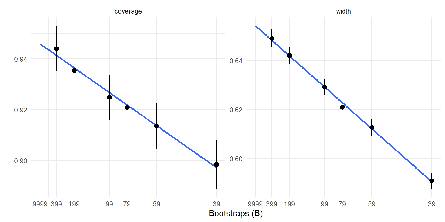
The graphs above suggest that linear extrapolation is quite reasonable, both for coverage and interval width. The graphs also show that both metrics are meaningfully affected by the number of bootstraps.
A literal approach to computing the extrapolated coverage rate and interval width is to fit a regression across all the replications and values of \(b\):
library(clubSandwich)
res$rep <- rep(1:2500, each = length(B_vals))

# coverage extrapolation
lm(coverage ~ I(1 / B), data = res) |>
  conf_int(vcov = "CR1", cluster = res$rep, test = "z", coefs = "(Intercept)")
Coef. Estimate SE d.f. Lower 95% CI Upper 95% CI
(Intercept) 0.946 0.00433 Inf 0.938 0.955# width extrapolation
lm(width ~ I(1 / B), data = res) |>
conf_int(vcov = "CR1", cluster = res$rep, test = "z", coefs = "(Intercept)") Coef. Estimate SE d.f. Lower 95% CI Upper 95% CI
(Intercept) 0.654 0.00182 Inf 0.651 0.658The calculation can be simplified a bit (or at least made a little more transparent?) by recognizing that \(\hat\alpha_0\) is a simple average of the intercepts from each block-specific regression (call these \(\hat\alpha_{0r}\) for \(r = 1,..,R\)) and that \(\hat\alpha_{0r}\) is just a weighted average of the outcomes, with weights determined by \(B_1,...,B_P\). The weights are given by \[ w_{br} = \frac{1}{p} - \frac{\tilde{B}}{S_B} \times \left(\frac{1}{b} - \tilde{B}\right), \] where \(\displaystyle{\tilde{B} = \frac{1}{p} \sum_{b \in \{B_1,...,B_P\}} \frac{1}{b}}\) and \(\displaystyle{S_B = \sum_{b \in \{B_1,...,B_P\}} \left(\frac{1}{b} - \tilde{B}\right)^2}\). With these weights, \[ \hat\alpha_{0r} = \sum_{b \in \{B_1,...,B_P\}} w_{br} C_{br} \] and \[ \hat\alpha_0 = \frac{1}{R} \sum_{r=1}^R \hat\alpha_{0r} \] with (cluster-robust) standard error \[ SE = \sqrt{\frac{1}{R} \times \frac{\sum_{r=1}^R \left(\hat\alpha_{0r} - \hat\alpha_0\right)^2}{R - 1}}. \] Here’s a function that does the above calculations:
calc_CI_coverage_width <- function(res, B_vals) {

  # calculate wts for each replication
  p <- length(B_vals)
  Btilde <- mean(1 / B_vals)
  x <- 1 / B_vals - Btilde
  S_B <- as.numeric(crossprod(x))
  B_wts <- 1 / p - x * Btilde / S_B

  res %>%
    group_by(rep) %>%
    # calculate alpha_0r per replication
    summarize(
      across(c(coverage, width), ~ sum(.x * B_wts)),
      .groups = "drop"
    ) %>%
    # average over replications
    summarize(
      across(c(coverage, width), list(
        M = ~ mean(.x),
        SE = ~ sd(.x) / sqrt(n())
      ))
    )

}

calc_CI_coverage_width(res, B_vals = B_vals)
# A tibble: 1 × 4
coverage_M coverage_SE width_M width_SE
<dbl> <dbl> <dbl> <dbl>
1 0.946 0.00433 0.654 0.00182Let’s see how the extrapolated coverage rate and interval width compare to the brute-force approach. I’ll do this by re-running the simulations using \(B = 2399\) booties, but not bothering with the extrapolation.
big_booties <- simulate_bootCIs(
  reps = 2500,
  N = 50,
  mu = 2,
  nu = 5,
  B_vals = 2399
)

big_sim_summary <-
  big_booties %>%
    summarize(
      across(c(coverage, width), list(
        M = ~ mean(.x),
        SE = ~ sd(.x) / sqrt(n())
      ))
    )

big_sim_summary
coverage_M coverage_SE width_M width_SE
1 0.9516 0.004293058 0.655017 0.001779658big_sim_summary %>%
mutate(B = 1999L) %>%
bind_rows(sim_summary) %>%
mutate(
est = if_else(B == 1999L, "Brute-force", "Extrapolation")
) %>%
pivot_longer(
c(ends_with("_M"), ends_with("_SE")),
names_to = c("metric", ".value"),
names_pattern = "(.+)_(.+)"
) %>%
ggplot() +
aes(x = B, y = M) +
scale_x_continuous(transform = "reciprocal", breaks = c(B_vals, 9999)) +
scale_color_manual(values = c(`Brute-force` = "red", `Extrapolation` = "black")) +
expand_limits(x = 9999) +
geom_smooth(aes(group = est), method = "lm", formula = y ~ x, fullrange = TRUE, se = FALSE, color = "grey") +
geom_pointrange(aes(ymin = M - qn * SE, ymax = M + qn * SE, color = est)) +
facet_wrap(~ metric, scales = "free") +
theme_minimal() +
theme(legend.position = c(0.9, 0.9)) +
labs(x = "Bootstraps (B)", y = "", color = "")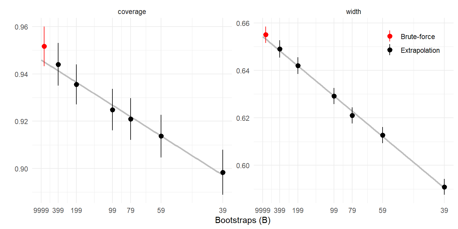
The extrapolated coverage rate and interval width are consistent with the brute-force calculations. The brute-force approach requires calculating \(2399 \times R\) booties, whereas the extrapolation requires only \(399 \times R\) booties. However, the number of confidence interval calculations is one per bootstrap, or \(2399 \times R\) in all for the brute-force calculation (in this example, that comes out to be 5,997,500), but \(399 \times R \times \left(m \times (P - 1) + 1\right)\) for the extrapolation approach (in this example, that comes out to 50,872,500). Thus, this technique is only going to be worth the trouble if computing the booties takes much longer than doing the confidence interval calculations.
The Boos & Zhang (2000) technique seems quite useful and worth knowing about if you’re doing any sort of Monte Carlo simulations involving bootstrapping. I’ve provided a proof-of-concept code-through, but there’s a certainly a few loose ends here. For one, what’s the right set of sub-sample bootie sizes? I’ve followed Boos and Zhang’s suggestion, but it’s not based on much of any theory. I’ve deviated a little bit from the original paper by using \(m\) repeated sub-samples instead of implementing the probability calculations proposed in the original paper. Is there a cost to this? Not sure. Is \(m = 10\) the right number to use? Again, not sure. Some further fiddling seems warranted.
This code-through also has me wondering about how the approach could be abstracted to make it easier to apply to new problems. It seems like the sort of thing that would fit well in simhelpers, but this will take a bit more thought.