---
title: Step-function selection models for meta-analysis
date: '2024-07-09'
categories:
- effect size
- distribution theory
- selective reporting
execute:
echo: false
bibliography: "../selection-references.bib"
csl: "../apa.csl"
link-citations: true
code-tools: true
toc: true
css: styles.css
crossref:
eq-prefix: ""
---
In [a recent post](/posts/distribution-of-significant-effects/) I looked at the distribution of statistically significant effect sizes in studies that report multiple outcomes, when those studies are subject to a certain form of selective reporting.
I considered a model where each effect size within the study is more likely to be reported when it is _affirmative_---or statistically significant and in the hypothesized direction---than when it is _non-affirmative_.
Because studies with multiple effect sizes are a very common occurrence in social science meta-analysis, it's interesting to think about how this form of selection leads to distortions of the results that are actually reported and available for meta-analysis.
In this post, I want to look a different scenario that is simpler in one respect but more complicated in another.
Simpler, in that I'm going to ignore dependence issues and just think about the distribution of one effect size at a time.
More complicated, in that I'm going to look at a more general model for how selective reporting occurs, which I'll call the __*step-function selection model*__.
# The step-function selection model
The step-function selection model was introduced by @hedges1992modeling and has been further expanded, tweaked, and studied in a bunch of subsequent work.
The model has two components: a set of assumptions about how effect size estimates are generated prior to selection (the _evidence-generation process_), and a set of assumptions about how selective reporting happens as a function of the effect size estimates (the _selective reporting process_).
In the original formulation, the evidence-generation process is a random effects model. Letting $T_i^*$ denote an effect size estimate prior to selective reporting and $\sigma_i^*$ denote its (known) standard error, we assume that
$$
T_i^* | \sigma_i^* \sim N\left(\mu, \tau^2 + \left(\sigma_i^*\right)^2\right),
$$ {#eq-evidence-generation}
just as in the conventional random effects model. Here $\mu$ is the overall average effect size and $\tau$ is the standard deviation of the effect size parameter distribution.
For the second component, we assume that the selective-reporting process is fully determined by the statistical significance and sign of the effect size estimates. We can therefore formalize the selective reporting process in terms of the one-sided p-values of the effect size estimates. Assuming that the degrees of freedom are large enough to not worry about, the one-sided p-value for effect size $i$ is a transformation of the effect size and its standard error:
$$
p_i^* = 1 - \Phi\left(T_i^* / \sigma_i^*\right)
$$ {#eq-p-onesided}
In the step-function model, we assume that the probability that an effect size estimate is reported (and thus available for meta-analysis) depends on where this one-sided p-value lies relative to a pre-specified set of significance thresholds, $\alpha_1,...,\alpha_H$. These thresholds define a set of intervals, each of which can have a different probability of selection.
Let $O_i^*$ be a binary indicator equal to 1 if $T_i^*$ is reported and otherwise equal to zero.
The selective reporting process is then
$$
\Pr\left(O_i^* = 1| T_i^*, \sigma_i^*\right) = \begin{cases}
1 & \text{if} \quad p_i^* < \alpha_1 \\
\lambda_1 & \text{if} \quad \alpha_h \leq p_i^* < \alpha_{h+1}, \quad h = 1,...,H-1 \\
\lambda_H & \text{if} \quad \alpha_H \leq p_i^* \\
\end{cases}.
$$ {#eq-selection-process}
Note that the selection probability for the lowest interval $[0, \alpha_1)$ is fixed to 1 because we can't estimate the absolute probability that an effect size estimate is reported.
The remaining parameters of the selection process therefore each represent a ratio of the probability of reporting an effect size estimate falling in a given interval to the probability of reporting an effect size estimate falling in the lowest interval.
In practice, the analyst will need to specify the thresholds of the significance intervals in order to estimate the model. One common choice is to use only a single threshold at $\alpha_1 = .025$, which corresponds to a two-sided level of .05---Fisher's vaunted criteria for when a result should be considered significant. This is the so-called "three-parameter" selection model, where the parameters of interest are the average effect size $\mu$, the heterogeneity SD $\tau$, and the relative selection probability $\lambda_1$. Other possible choices for thresholds might be:
* A single threshold at $\alpha_1 = .50$, so that negatively-signed effect size estimates have a different selection probability than positively-signed estimates;
* A two-threshold model with $\alpha_1 = .025$ and $\alpha_2 = .50$ (I like to call this a four-parameter selection model); or
* A model with thresholds for significant, positive results at $\alpha_1 = .025$, for the sign of the estimate at $\alpha_2 = .50$, and for statistically significant results in the opposite of the expected direction at $\alpha_3 = .975$.
Many other choices are possible, of course.
# Distribution of observed effect sizes
Equations (@eq-evidence-generation) and (@eq-selection-process) are sufficient to describe the distribution of effect sizes actually observed after selection. If we let $T_i$ and $\sigma_i$ denote effect size estimates that are actually observed, then the distribution of $\left(T_i | \sigma_i\right)$ is the same as that of $\left(T_i^* | \sigma_i^*, O_i^* = 1\right)$. By Bayes Theorem,
$$
\Pr(T_i = t | \sigma_i) = \frac{\Pr\left(O_i^* = 1| T_i^* = t, \sigma_i^* = \sigma_i\right) \times \Pr(T_i^* = t| \sigma_i^* = \sigma_i)}{\Pr\left(O_i^* = 1| \sigma_i^* = \sigma_i\right)}
$$ {#eq-observed-effect-distribution}
For the specific distributional assumptions of the step-function selection model, we can find an expression for the exact form of (@eq-observed-effect-distribution).
In doing so, it will be useful to define a further random variable---call it $S_i$---that is equal to the p-value interval into which effect size $T_i$ falls. For a given effect size with standard error $\sigma_i^*$, these intervals are equivalent to intervals on the scale of the outcome, with thresholds $\gamma_{hi} = \sigma_i^* \Phi^{-1}(1 - \alpha_h)$. Now, let's define $S_i^*$ as
$$
S_i^* = \begin{cases}
0 & \text{if} \quad \gamma_{1i} < T_i^* \\
h & \text{if} \quad \gamma_{h+1,i} < T_i^* \leq \gamma_{hi}, \quad h = 1,...,H-1 \\
H & \text{if} \quad T_i^* \leq \gamma_{Hi} \\
\end{cases}
$$
and $S_i$ as the corresponding interval for the observed effect size $T_i$.
Note that (@eq-selection-process) is equivalent to writing the relative selection probabilities as a function of $S_i$:
$$
w\left(T_i^*, \sigma_i^*\right) = \lambda_{S_i^*}
$$ {#eq-selection-weights}
Also note that, prior to selection, the effect size estimate $T_i^*$ has marginal variance $\eta_i^2 = \tau^2 + \left(\sigma_i^*\right)^2$, so we can write $\Pr(T_i^* = t| \sigma_i^*) = \frac{1}{\eta_i}\phi\left(\frac{t - \mu}{\eta_i}\right)$, where $\phi()$ is the standard normal density. We can then write the distribution of the observed effect size estimates as
$$
\Pr(T_i = t | \sigma_i) = \frac{w\left(t, \sigma_i\right) \times \frac{1}{\eta_i}\phi\left(\frac{t - \mu}{\eta_i}\right)}{A_i},
$$ {#eq-observed-effect-density}
where
$$
\begin{aligned}
A_i &= \int w\left(t, \sigma_i^*\right) \times \frac{1}{\eta_i}\phi\left(\frac{t - \mu}{\eta_i}\right) dt \\
&= \sum_{h=0}^H \lambda_h B_{hi},
\end{aligned}
$$ {#eq-Ai}
with
$$
B_{hi} = \Phi\left(\frac{\gamma_{hi} - \mu}{\eta_i}\right) - \Phi\left(\frac{\gamma_{h+1,i} - \mu}{\eta_i}\right)
$$
and where we take $\lambda_0 = 1$, $\alpha_0 = 0$, and $\alpha_{H+1} = 1$ [@hedges2005selection]. Note that $A_i = \Pr(O^* = 1 | \sigma_i^*)$, the probability that an effect size estimate with precision $\sigma_i^*$ will be observed.
The observed effect size estimates follow what we might call a "piece-wise normal" distribution.
For a given $\sigma_i$ and given the interval $S_i$ into which the effect size falls, the effect size follows a truncated normal distribution. Formally,
$$
\left(T_i | S_i = h, \sigma_i \right) \sim TN(\mu,\eta_i^2, \gamma_{h+1,i},\gamma_{h i}).
$$
Furthermore, the distribution of $S_i$ is given by
$$
\Pr(S_i = h | \sigma_i) = \frac{\lambda_h B_{hi}}{\sum_{g=0}^H \lambda_g B_{gi}},
$$
which will be useful for deriving moments of the distribution of $T_i$.
Here is an interactive graph showing the distribution of the effects prior to selection (in grey) and the distribution of observed effect sizes (in blue) based on a four-parameter selection model with selection thresholds of $\alpha_1 = .025$ and $\alpha_2 = .50$. Initially, the selection parameters are set to $\lambda_1 = 0.6$ and $\lambda_2 = 0.3$, but you can change these however you like.
```{ojs}
math = require("mathjs")
norm = import('https://unpkg.com/norm-dist@3.1.0/index.js?module')

eta = math.sqrt(tau**2 + sigma**2)
H = 2
alpha = [.025, .500]
lambda = [1, lambda1, lambda2]
lambda_max = math.max(lambda)

function findlambda(p, alp, lam) {
  var m = 0;
  while (p >= alp[m]) {
    m += 1;
  }
  return lam[m];
}

function findMoments(mu, tau, sigma, alp, lam) {
  let H = alp.length;
  let eta = math.sqrt(tau**2 + sigma**2);

  let gamma_h = Array(H+2).fill(null).map((x,i) => {
    if (i==0) {
      return Infinity;
    } else if (i==H+1) {
      return -Infinity;
    } else {
      return sigma * norm.icdf(1 - alp[i-1]);
    }
  });

  let c_h = Array(H+2).fill(null).map((x,i) => {
    return (gamma_h[i] - mu) / eta;
  });

  let B_h = Array(H+1).fill(null).map((x,i) => {
    return norm.cdf(c_h[i]) - norm.cdf(c_h[i+1])
  });

  let Ai = 0;
  for (let i = 0; i <= H; i++) {
    Ai += lam[i] * B_h[i];
  }

  let psi_h = Array(H+1).fill(null).map((x,i) => {
    return (norm.pdf(c_h[i+1]) - norm.pdf(c_h[i])) / B_h[i]
  });

  let psi_top = 0;
  for (let i = 0; i <= H; i++) {
    psi_top += lam[i] * B_h[i] * psi_h[i];
  }

  let psi_bar = psi_top / Ai;

  let ET = mu + eta * psi_bar;

  let dc_h = c_h.map((c_val) => {
    if (math.abs(c_val) == Infinity) {
      return 0;
    } else {
      return c_val * norm.pdf(c_val);
    }
  });

  let kappa_h = Array(H+1).fill(null).map((x,i) => {
    return (dc_h[i] - dc_h[i+1]) / B_h[i];
  });

  let kappa_top = 0;
  for (let i = 0; i <= H; i++) {
    kappa_top += lam[i] * B_h[i] * kappa_h[i];
  }
  let kappa_bar = kappa_top / Ai;
  let SDT = eta * math.sqrt(1 - kappa_bar - psi_bar**2);

  return ({Ai: Ai, ET: ET, SDT: SDT});
}

moments = findMoments(mu, tau, sigma, alpha, lambda)
Ai_toprint = moments.Ai.toFixed(3)
ET_toprint = moments.ET.toFixed(3)
eta_toprint = eta.toFixed(3)
SDT_toprint = moments.SDT.toFixed(3)
```
```{ojs}
pts = 201

dat = Array(pts).fill().map((element, index) => {
  let t = mu - 3 * eta + index * eta * 6 / (pts - 1);
  let p = 1 - norm.cdf(t / sigma);
  let dt = norm.pdf((t - mu) / eta) / eta;
  let lambda_val = findlambda(p, alpha, lambda);
  return ({
    t: t,
    d_unselected: dt,
    d_selected: lambda_val * dt / lambda_max
  })
})
```
::::: {.grid .column-page}
:::: {.g-col-8 .center}
```{ojs}
Plot.plot({
  height: 300,
  width: 700,
  y: {
    grid: false,
    label: "Density"
  },
  x: {
    label: "Effect size estimate (Ti)"
  },
  marks: [
    Plot.ruleY([0]),
    Plot.ruleX([0]),
    Plot.areaY(dat, {x: "t", y: "d_unselected", fillOpacity: 0.3}),
    Plot.areaY(dat, {x: "t", y: "d_selected", fill: "blue", fillOpacity: 0.5}),
    Plot.lineY(dat, {x: "t", y: "d_selected", stroke: "blue"})
  ]
})
```
:::{.moments}
```{ojs}
tex`
\begin{aligned}
\mu &= ${mu} & \qquad \eta_i &= ${eta_toprint} \\
\mathbb{E}\left(T_i\right) &= ${ET_toprint}
& \qquad \sqrt{\mathbb{V}\left(T_i\right)} &= ${SDT_toprint} \\
\Pr(O_i^* = 1) &= ${Ai_toprint}
\end{aligned}
`
```
:::
::::
:::: {.g-col-4}
```{ojs}
//| panel: input
viewof mu = Inputs.range(
  [-2, 2],
  {value: 0.15, step: 0.01, label: tex`\mu`}
)

viewof tau = Inputs.range(
  [0, 2],
  {value: 0.10, step: 0.01, label: tex`\tau`}
)

viewof sigma = Inputs.range(
  [0, 1],
  {value: 0.20, step: 0.01, label: tex`\sigma_i`}
)

viewof lambda1 = Inputs.range(
  [0, 2],
  {value: 0.60, step: 0.01, label: tex`\lambda_1`}
)

viewof lambda2 = Inputs.range(
  [0, 2],
  {value: 0.30, step: 0.01, label: tex`\lambda_2`}
)
```
::::
:::::
# Moments of $T_i | \sigma_i$
Using the auxiliary random variable $S_i$ makes it pretty straight-forward to find the moments of $T_i | \sigma_i$. Let me denote
$$
\psi_{hi} = \frac{\phi\left(c_{h+1,i}\right) - \phi\left(c_{hi}\right)}{B_{hi}},
$$
where $c_{hi} = \left(\gamma_{hi} - \mu\right) / \eta_i$ for $h=0,...,H$.
Then from the properties of truncated normal distributions,
$$
\mathbb{E}(T_i | S_i = h, \sigma_i) = \mu + \eta_i \times \psi_{hi},
$$
It follows immediately that
$$
\begin{aligned}
\mathbb{E}(T_i | \sigma_i) &= \sum_{h=0}^H \Pr(S_i = h | \sigma_i) \times \mathbb{E}(T_i | S_i = h, \sigma_i) \\
&= \mu + \eta_i \frac{\sum_{h=0}^H \lambda_h B_{hi} \psi_{hi}}{\sum_{h=0}^H \lambda_h B_{hi}}.
\end{aligned}
$$ {#eq-Ti-expectation}
The second term of (@eq-Ti-expectation) is the bias of $T_i$ relative to the overall mean effect $\mu$. Generally, it will depend on all the parameters of the evidence-generating process, including $\sigma_i$, $\mu$, and $\tau$ (through the $c_{hi}$ and $B_{hi}$ terms) and on the selection weights $\lambda_1,...,\lambda_H$.
Just for giggles, let me chug through and get the variance of $T_i$ as well. Letting
$$
\bar\psi_i = \frac{\sum_{h=0}^H \lambda_h B_{hi} \psi_{hi}}{\sum_{h=0}^H \lambda_h B_{hi}}
$$
and
$$
\kappa_{hi} = \frac{c_{hi} \phi\left(c_{hi}\right) - c_{h+1,i} \phi\left(c_{h+1,i}\right)}{B_{hi}},
$$
we can write the variance of the truncated normal conditional distribution
$$
\mathbb{V}(T_i | S_i = h, \sigma_i) = \eta_i^2 \left(1 - \kappa_{hi} - \psi_{hi}^2\right).
$$
Using variance decomposition, we then have
$$
\begin{aligned}
\mathbb{V}(T_i | \sigma_i) &= \mathbb{E}\left[\mathbb{V}(T_i | S_i, \sigma_i)\right] + \mathbb{V}\left[\mathbb{E}(T_i | S_i, \sigma_i)\right] \\
&= \mathbb{E}\left[\mathbb{V}(T_i | S_i, \sigma_i) + \left[\mathbb{E}(T_i | S_i, \sigma_i) - \mathbb{E}(T_i | \sigma_i)\right]^2\right] \\
&= \frac{1}{\sum_{h=0}^H \lambda_h B_{hi}} \sum_{h=0}^H \lambda_h B_{hi} \left( \eta_i^2 \left(1 - \kappa_{hi} - \psi_{hi}^2\right) + \eta_i^2 \left[\psi_{hi} - \bar\psi_i \right]^2\right) \\
&= \eta_i^2 \left(1 - \bar\kappa_i - \bar\psi_i^2\right),
\end{aligned}
$$ {#eq-Ti-variance}
where
$$
\bar\kappa_i = \frac{\sum_{h=0}^H \lambda_h B_{hi} \kappa_{hi}}{\sum_{h=0}^H \lambda_h B_{hi}}
$$
Just as with the expectation, the variance is a complicated function of all the model parameters.
# Funnel density
The graph above shows the distribution of observed effect size estimates with a given sampling standard error $\sigma_i$.
In practice, meta-analysis datasets include many effect sizes with a range of different standard errors.
Funnel plots are a commonly used graphical representation the distribution of effects in a meta-analysis.
They are simply scatterplots, showing effect size estimates on the horizontal axis and standard errors (or some measure of precision) on the vertical axis.
Usually, they are arranged so that effects from larger studies appear closer to the top of the plot.
Funnel plots are often used a diagnostic for selective reporting because they will tend to be asymmetric when non-affirmative effects are less likely to be reported than affirmative effects.
I think it's pretty useful to use the layout of a funnel plot to understand how meta-analytic models work. A basic random effects model implies a certain distribution of population effects, which can be represented by the density of points in a funnel plot.[^technically-conditional]
That density will have a shape kind of like an upside down funnel: narrow near the top (where studies are large and $\sigma_i$ is small), getting wider and wider as $\sigma_i$ increases (i.e., as studies get smaller and smaller).
[^technically-conditional]: To be precise, the density will depend on the marginal distribution of $\sigma_i^*$'s in the population of effects. I'm going to side-step this problem by using the funnel plot layout to show the _conditional_ distribution of the effect size estimates, given $\sigma_i^* = \sigma_i$.
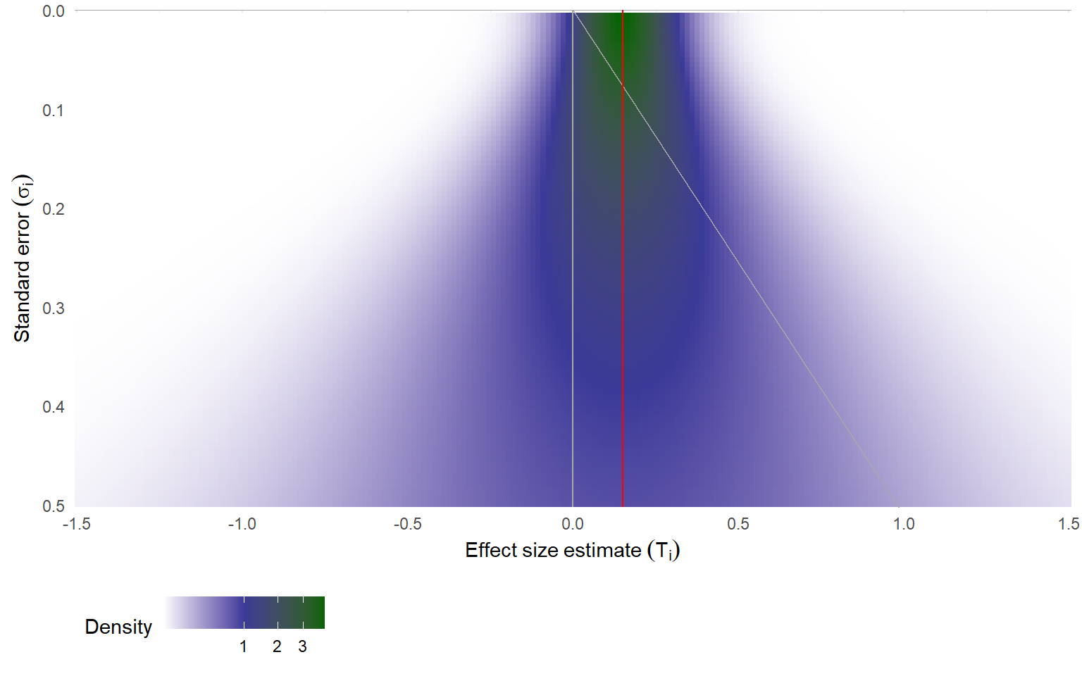
Here's an illustration of this density, using darker color to indicate areas of the plot where effect sizes are more likely.
I've used $\mu = 0.15$ (represented by the vertical red line) and $\tau = 0.10$ to calculate the density.
The vertical gray line corresponds to $\mu = 0$, which is also the threshold where effect size estimates will have $p$-values of $\alpha = .50$.
The sloped gray line corresponds to the treshold where effect size estimates have $p$-values of $\alpha = .025$; to the right of this line, effects will be statistically significant and affirmative; to the left, effects are non-affirmative.
```{r}
#| fig-width: 8
#| fig-height: 5
#| out-width: 90%
library(tidyverse)
mu <- 0.15
tau <- 0.10
dat <-
expand_grid(
t = seq(-1.5, 1.5, length.out = 201),
se = seq(0.005, 0.500, 0.005)
) %>%
mutate(
eta = sqrt(tau^2 + se^2),
dt = dnorm(t, mean = mu, sd = eta)
)
ggplot(dat, aes(t, se, fill = dt)) +
geom_tile() +
geom_hline(yintercept = 0, color = "darkgrey") +
geom_vline(xintercept = 0, color = "darkgrey") +
geom_abline(intercept = 0, slope = -1 / qnorm(0.975), color = "darkgrey") +
geom_vline(xintercept = mu, color = "red") +
scale_fill_gradient2(
transform = "sqrt",
low = "white",
mid = scales::muted("blue"),
high = "darkgreen",
midpoint = 1
) +
scale_y_reverse() +
coord_cartesian(expand = FALSE) +
theme_minimal() +
theme(legend.position = "bottom", legend.justification.bottom = "left") +
labs(
x = expression(Effect~size~estimate~(T[i])),
y = expression(Standard~error~(sigma[i])),
fill = "Density"
)
```
The above graph shows the (conditional) distribution of effect size estimates under the random effects model, without any selective reporting.
Selective reporting of study results will distort this distribution, shrinking the density for effects that are not affirmative.
Here is an interactive funnel plot showing the distribution of effect size estimates under a four-parameter selection model. Just as in the interactive graph above, I use fixed selection thresholds of $\alpha_1 = .025$ and $\alpha_2 = .50$. Initially, I set $\mu = 0.15$ and $\tau = 0.10$ and selection parameters of $\lambda_1 = 0.6$ and $\lambda_2 = 0.3$, but you can change these however you like.
```{ojs}
SE_pts = 100
t_pts = 181
lambda_f = [1, lambda1_f, lambda2_f]
alpha_f = [.025, .500]
sigma_max = 0.5
eta_max_f = math.sqrt(tau_f**2 + sigma_max**2)

funnel_dat = Array(t_pts * SE_pts).fill(null).map((x,row) => {
  let i = row % SE_pts;
  let j = (row - i) / SE_pts;
  let sigma = (i + 1) * sigma_max / SE_pts;
  let t = mu_f - 3 * eta_max_f + j * eta_max_f * 6 / (t_pts - 1);
  let eta = math.sqrt(tau_f**2 + sigma**2);
  let p = 1 - norm.cdf(t / sigma);
  let dt = norm.pdf((t - mu_f) / eta) / eta;
  let lambda_val = findlambda(p, alpha_f, lambda_f);
  return ({i: i, j: j, t: t, sigma: sigma, eta: eta, p: p, dt: dt, lambda: lambda_val, d_selected: lambda_val * dt});
})

sigline_dat = [
  ({t: 0, sigma: 0}),
  ({t: sigma_max * norm.icdf(0.975), sigma: sigma_max})
]
```
::::: {.grid .column-page}
:::: {.g-col-8 .center}
```{ojs}
Plot.plot({
  height: 400,
  width: 700,
  padding: 0,
  grid: false,
  x: {axis: "top", label: "Effect size estimate (Ti)"},
  y: {label: "Standard error (sigma_i)", reverse: true},
  color: {
    scheme: "pubugn",
    type: "sqrt",
    label: "Density"
  },
  marks: [
    Plot.dot(funnel_dat, {x: "t", y: "sigma", fill: "d_selected", r:2, symbol: "square"}),
    Plot.ruleY([0], {stroke: "black"}),
    Plot.ruleX([0], {stroke: "grey"}),
    Plot.line(sigline_dat, {x: "t", y: "sigma", stroke: "gray", strokeWidth: 1})
  ]
})
```
```{ojs}
Plot.legend({color: {scheme: "pubugn", type: "sqrt", label: "Density"}})
```
::::
:::: {.g-col-4}
```{ojs}
//| panel: input
viewof mu_f = Inputs.range(
  [-2, 2],
  {value: 0.15, step: 0.01, label: tex`\mu`}
)

viewof tau_f = Inputs.range(
  [0, 2],
  {value: 0.10, step: 0.01, label: tex`\tau`}
)

viewof lambda1_f = Inputs.range(
  [0, 2],
  {value: 0.60, step: 0.01, label: tex`\lambda_1`}
)

viewof lambda2_f = Inputs.range(
  [0, 2],
  {value: 0.30, step: 0.01, label: tex`\lambda_2`}
)
```
::::
:::::
If you fiddle with the selection parameters, you will see that the density of certain areas of the plot changes.
For instance, lowering $\lambda_2$ will reduce the density of negative effect size estimates; lowering $\lambda_1$ will reduce the density of positive but non-affirmative effect size estimates, which fall between the vertical axis and the diagonal line corresponding to $\alpha = .025$.
# Comment
In this post, I've given expressions for the density of effect size estimates under the step-function selection model, as well as expressions for the mean and variance of effect size estimates of a given precision (i.e., for $T_i | \sigma_i$).
Although these expressions are pretty complex, it seems like they could be useful for studying the properties of different estimators that have been proposed for dealing with selective reporting, such as the "unrestricted weighted least squares" method, which is just the idea of using fixed effects weights even though the effects are heterogeneous [@henmi2010confidence; @stanley2014metaregression]; the PET and PEESE estimators [@stanley2008metaregression]; the endogenous kink meta-regression [@bom2019kinked]; and perhaps other estimators in the literature.
Graphical depictions of the step function density (as in the funnel plot above) also seem potentially useful for understanding the properties of these estimators.